Unfolding Local Growth Rate Estimates

for (Almost) Perfect Adversarial Detection

Peter Lorenz

, Margret Keuper

2,3

and Janis Keuper

1,4

ITWM Fraunhofer, Kaiserslautern, Germany

University of Siegen, Germany

Max Planck Institute for Informatics, Saarland Informatics Campus, Saarbr

ucken, Germany

IMLA, Offenburg University, Germany

Keywords:

Adversarial Examples, Detection.

Abstract:

Convolutional neural networks (CNN) deﬁne the state-of-the-art solution on many perceptual tasks. However,

current CNN approaches largely remain vulnerable against adversarial perturbations of the input that have

been crafted speciﬁcally to fool the system while being quasi-imperceptible to the human eye. In recent years,

various approaches have been proposed to defend CNNs against such attacks, for example by model hardening

or by adding explicit defence mechanisms. Thereby, a small “detector” is included in the network and trained

on the binary classiﬁcation task of distinguishing genuine data from data containing adversarial perturbations.

In this work, we propose a simple and light-weight detector, which leverages recent ﬁndings on the relation

between networks’ local intrinsic dimensionality (LID) and adversarial attacks. Based on a re-interpretation

of the LID measure and several simple adaptations, we surpass the state-of-the-art on adversarial detection by

a signiﬁcant margin and reach almost perfect results in terms of F1-score for several networks and datasets.

Sources available at: https://github.com/adverML/multiLID

1 INTRODUCTION

Deep Neural Networks (DNNs) are highly expres-

sive models that have achieved state-of-the-art perfor-

mance on a wide range of complex problems, such

as in image classiﬁcation. However, studies have

found that DNN’s can easily be compromised by ad-

versarial examples (Goodfellow et al., 2015; Madry

et al., 2018; Croce and Hein, 2020a; Croce and Hein,

2020b). Applying these intentional perturbations to

network inputs, chances of potential attackers to fool

target networks into making incorrect predictions at

test time are very high (Carlini and Wagner, 2017a).

Hence, this undesirable property of deep networks has

become a major security concern in real-world appli-

cations of DNNs, such as self-driving cars and iden-

tity recognition (Evtimov et al., 2017; Sharif et al.,

2019).

Recent research on adversarial counter measures

can be grouped into two main approach angles: ad-

versarial training and adversarial detection. While the

ﬁrst group of methods aims to ”harden” the robustness

of networks by augmenting the training data with ad-

versarial examples, the later group tries to detect and

reject malignant inputs.

In this paper, we restrict our investigation to the

detection of adversarial images exposed to convolu-

tional neural networks (CNN). We introduce a novel

white-box detector, showing a close to perfect de-

tection performance on widely used benchmark set-

tings. Our method is built on the notion that adver-

sarial samples are forming distinct sub-spaces, not

only in the input domain but most dominantly in the

feature spaces of neural networks (Szegedy et al.,

2014). Hence, several prior works have attempted to

ﬁnd quantitative measures for the characterization and

identiﬁcation of such adversarial regions. We investi-

gate the properties of the commonly used local intrin-

sic dimensionality (LID) and show that a robust iden-

tiﬁcation of adversarial sub-spaces requires (i) an un-

folded local representation and (ii) a non-linear sepa-

ration of these manifolds. We utilize these insights to

formulate our novel multiLID descriptor. Extensive

experimental evaluations of the proposed approach

show that multiLID allows a reliable identiﬁcation of

adversarial samples generated by state-of-the art at-

tacks on CNNs. In summary, our contributions are:

Lorenz, P., Keuper, M. and Keuper, J.

Unfolding Local Growth Rate Estimates for (Almost) Perfect Adversarial Detection.

DOI: 10.5220/0011586500003417

In Proceedings of the 18th International Joint Conference on Computer Vision, Imaging and Computer Graphics Theory and Applications (VISIGRAPP 2023) - Volume 5: VISAPP, pages

27-38

ISBN: 978-989-758-634-7; ISSN: 2184-4321

 2023 by SCITEPRESS – Science and Technology Publications, Lda. Under CC license (CC BY-NC-ND 4.0)

• an analysis of the widely used LID detector.

• novel re-formulation of an unfolded, non-linear

multiLID descriptor which allows a close to per-

fect detection of adversarial input images in CNN

architectures.

• in-depth evaluation of our approach on common

benchmark architectures and datasets, showing

the superior performance of the proposed method.

2 RELATED WORK

In the following, we ﬁrst brieﬂy review the related

work on adversarial attacks and provide details on the

established attack approaches that we base our evalu-

ation on. Then, we summarize approaches to network

hardening by adversarial training. Last, we revise the

literature on adversarial detection.

2.1 Adversarial Attacks

Convolutional neural networks are known to be

susceptible to adversarial attacks, i.e. to (usually

small) perturbation of the input images that are

optimized to ﬂip the network’s decision. Several such

attacks have been proposed in the past and we base

our experimental evaluation on the following subset

of most widely used attacks.

Fast Gradient Method (FGSM) (Goodfellow et al.,

2015): uses the gradients of a given model to cre-

ate adversarial examples, i.e. it is a white-box attack

and needs full access to the model architecture and

weights. It maximizes the model’s loss J w.r.t. the in-

put image via gradient ascent to create an adversarial

image X

adv

= X + ε · sign(∇

J(X

adv

)) ,

where X is the benign input image, y is the image

label, and ε is a small scalar that ensures the pertur-

bations are small.

Basic Iterative Method (BIM) (Kurakin et al.,

2017): is an improved, iterative version of FGSM.

After each iteration the pixel values are clipped to the

ε ball around the input image (i.e. [x−ε,x+ε]) as well

as the input space (i.e. [0, 255] for the pixel values):

adv

= X,

adv

N+1

= CLIP

X,ε

adv

+ α ·sign(∇

J(X,y

))},

for iteration N with step size α.

Projected Gradient Descent (PGD) (Madry

et al., 2018): is similar to BIM and one of the

currently most popular attacks. PGD adds random

initializations of the perturbations for each iteration.

Optimized perturbations are again projected onto the

ε ball to ensure the similarity between original and

attacked image in terms of L

or L

∞

norm.

AutoAttack (AA) (Croce and Hein, 2020b): is an en-

semble of four parameter-free attacks: two parameter-

free variants of PGD (Madry et al., 2018) using cross-

entropy loss in APGD-CE and difference of logits

ratio loss (DLR) in APGD-t:

DLR(x,y) =

− max

x̸=y

π1

− z

π3

. (1)

where π is the ordering of the components of z in

decreasing order. Further AA comprises a targeted

version of the FAB attack (Croce and Hein, 2020a),

and the Squares attack (Andriushchenko et al.,

2020) which is a black-box attack. In RobustBench,

models are evaluated using AA in the standard mode

where the four attacks are executed consecutively.

If a sample’s prediction can not be ﬂipped by one

attack, it is handed over to the next attack method, to

maximize the overall attack success rate.

DeepFool (DF) : is a non-targeted attack that ﬁnds

the minimal amount of perturbation required to ﬂip

the networks decision by an iterative linearization

approach (Moosavi-Dezfooli et al., 2016). It thus

estimates the distance from the input sample to the

model decision boundary.

Carlini&Wagner (CW) (Carlini and Wagner,

2017b): uses a direct numerical optimization of

inputs X

adv

such as to ﬂip the network’s prediction at

minimum required perturbation and provides results

optimized with respect to L

, L

and L

∞

distances. In

our evaluation, we use the L

distance for CW.

Adversarial Training : denotes the concept of using

adversarial examples to augment the training data of

a neural network. Ideally, this procedure should lead

to a better and denser coverage of the latent space and

thus to in increased model robustness. FGSM (Good-

fellow et al., 2015) adversarial training offers the ad-

vantage of rather fast adversarial training data gener-

ation. Yet, models tend to overﬁt to the speciﬁc attack

such that additional tricks like early stopping (Rice

et al., 2020; Wong et al., 2020) have to be employed.

Training on multi-step adversaries generalizes more

easily, yet is hardly affordable for large-scale prob-

lems such as ImageNet due to its computation costs.

VISAPP 2023 - 18th International Conference on Computer Vision Theory and Applications

2.2 Adversarial Detection

Adversarial Detection aims to distinguish adversarial

examples from benign examples and is thus a low

computational replacement to expensive adversarial

training strategy. In test scenarios, adversarial attacks

can be rejected and cause to faulty classiﬁcations.

Given a trained DNN on a clean dataset for the origin

task, many existing methods (Ma et al., 2018; Fein-

man et al., 2017; Lee et al., 2018; Harder et al., 2021;

Lorenz et al., 2021) train a binary classiﬁer on top

of some hidden-layer embeddings of the given net-

work as the adversarial detector. The strategy is mo-

tivated by the observation that adversarial examples

have very different distribution from natural exam-

ples on intermediate-layer features. So a detector can

be built upon some statistics of the distribution, i.e.,

Kernel Density (KD) (Feinman et al., 2017), Maha-

lanobis Distance (MD) (Lee et al., 2018) distance,

or Local Intrinsic Dimensionality (LID) (Ma et al.,

2018). Spectral defense approaches (Harder et al.,

2021; Lorenz et al., 2021; Lorenz et al., 2022) aim

to detect adversarial images by their frequency spec-

tra in the input or feature map representation.

Complementary, (Yang et al., 2021) propose to train

a variational autoencoder following the principle of

the class distanglement. They argue that the recon-

structions of adversarial images are characteristically

different and can more easily be detected using for

example KD, MD and LID).

Local Intrinsic Dimensionality (LID): is a measure

that represents the average distance from a point to

its neighbors in a learned representation space (Am-

saleg et al., 2015; Houle, 2017a) and thereby approx-

imates the intrinsic dimensionality of the representa-

tion space via maximum likelihood estimation.

Let B be a mini-batch of N clean examples and Let

(x) = d(x,y) be the Euclidean distance between the

sample x and its i-th nearest neighbor in B. Then, the

LID can be approximated by

LID(x) = −

∑

i=1

log

(x)

−1

, (2)

where k is a hyper-parameter that controls the num-

ber of nearest neighbors to consider, and d is the em-

ployed distance metric. Ma et al.(Ma et al., 2018)

propose to use LID to characterize properties of ad-

versarial examples, i.e. they argue that the average

distance of samples to their neighbors in the learned

latent space of a classiﬁer is characteristic for adver-

sarial and benign samples. Speciﬁcally, they evaluate

LID for the j-dimensional latent representations of a

neural network f (x) of a sample x use the L

distance

ℓ

(x,y) = ∥ f

1.. j

ℓ

(x) − f

1.. j

ℓ

(y)∥

(3)

for all ℓ ∈ L feature maps. They compute a vector of

LID values for each sample:

−−→

LID(x) = {LID

ℓ

(x)}

ℓ

. (4)

Finally, they compute the

−−→

LID(x) over the training

data and adversarial examples generated on the train-

ing data, and train a logistic regression classiﬁer to

detect adversarial

samples.

3 REVISITING LOCAL

INTRINSIC DIMENSINALITY

The LID method for adversarial example detection as

proposed in (Ma et al., 2018) was motivated by the

MLE estimate for the intrinsic dimension as proposed

by (Amsaleg et al., 2015). We refer to this original

formulation to motivate our proposed multiLID.

Let us denote R

,d a continuous domain with

non-negative distance function d. The continuous

intrinsic dimensionality aims to measure the local

intrinsic dimensionality of R

in terms of the distri-

bution of inter point distances. Thus, we consider

for a ﬁxed point x the distribution of distances as

a random variable D on [o,+∞) with probability

density function f

and cumulative density function

. For samples x drawn from continuous probability

distributions, the intrinsic dimensionality is then

deﬁned as in (Amsaleg et al., 2015):

Deﬁnition 3.1. Instrinsic Dimensionality (ID). Given

a sample x ∈ R

, let D be a random variable denot-

ing the distance from x to other data samples. If the

cumulative distribution F(d) of D is positive and con-

tinuously differentiable at distance d > 0, the ID of x

at distance d is given by:

(d)

∆

= lim

ε→0

logF

((1 + ε)d) − logF

(d)

log(1 + ε)

(5)

In practice, we are given a ﬁxed number n of samples

of x such that we can compute their distances to x in

ascending order d

≤ d

≤ · ·· ≤ d

n−1

with maximum

distance w between any two samples. As shown in

(Amsaleg et al., 2015), the log-likelihood of ID

(d)

for x is then given as

nlog

D,w

(w)

+ nlogID

+ (ID

− 1)

n−1

∑

i=1

log

. (6)

We are grateful to the authors for releasing their

complete source code. https://github.com/xingjunm/lid

adversarial subspace detection.

Unfolding Local Growth Rate Estimates for (Almost) Perfect Adversarial Detection

The maximum likelihood estimate is then given as

= −

n−1

∑

i=0

log

−1

with (7)

∼ N





, (8)

i.e. the estimate is drawn from a normal distribu-

tion with mean ID

and its variance decreases linearly

with increasing number of samples while it increases

quadratically with ID

. The local ID is then an es-

timate of the ID based on the local neighborhood of

x, for example based on its k nearest neighbors. This

corresponds to equation (2). This local approximation

has the advantage of allowing for an efﬁcient compu-

tation even on a per batch basis as done in (Ma et al.,

2018). It has the disadvantage that is does not con-

sider the strong variations in variances ID

/n, i.e. the

estimates might become arbitrarily poor for large ID

if the number of samples is limited. This becomes

even more severe as (Amsaleg et al., 2021) showed

that latent representations with large ID are particu-

larly vulnerable to adversarial attacks.

In ﬁg. 1, we evaluate the distribution of LID esti-

mates computed for benign and adversarial examples

of different attacks on the latent feature representation

of a classiﬁer network (see section 4). We make the

following two observations: (i) the distribution has a

rather long tail and is not uni-modal, i.e. we are likely

to face rather strong variations in the ID for differ-

ent latent sub-spaces, (ii) the LID estimates for adver-

sarial examples have the tendency to be higher than

the ones for benign examples, (iii) the LID is more

informative for some attacks and less informative on

others. As a ﬁrst conclusion, we expect the discrimi-

nation between adversarial examples and benign ones

to be particularly hard when the tail of the distribution

is concerned, i.e. for those benign points with rather

large LID that can only be measured at very low conﬁ-

dence according to equation (7). Secondly, we expect

linear separation methods based on LID such as sug-

gested by (Ma et al., 2018) to be unnecessarily weak

and third, we expect the choice of the considered lay-

ers to have a rather strong inﬂuence on the expressive-

ness of LID for adversarial detection.

As a remedy, we propose several rather simple im-

provements:

• We propose to unfold the aggregated LID esti-

mates in equation (2) and rather consider the nor-

malized log distances between a sample and its

neighbors separately in a feature vector, which we

denote multiLID.

• We argue that the deep network layers considered

to compute LID or multiLID have to be carefully

chosen. An arbitrary choice might yield poor re-

sults.

• Instead of using a logistic regression classiﬁer,

highly non-linear classiﬁers such as a random for-

est should increase LID based discrimination be-

tween adversarial and benign samples.

Let us analyze the implications of the LID un-

folding in more detail. As argued for example in

(Ma et al., 2018) before, the empirically computed

LID can be interpreted as an estimate of the local

growth rate similarly to previous generalized expan-

sion models (Karger and Ruhl, 2002; Houle et al.,

2012). Thereby, the idea is to deduce the expansion

dimension from the volume growth around a sample

and the growth rate is estimated by considering prob-

ability mass in increasing distances from the sample.

Such expansion models, like the LID, are estimated

within a local neighborhood around each sample and

therefore provide a local view of the data dimension-

ality (Ma et al., 2018). The local ID estimation in

eq. (2) can be seen as a statistical interpretation of a

growth rate estimate. Please refer to (Houle, 2017a;

Houle, 2017b) for more details.

In practical settings, this statistical estimate not

only depends on the considered neighborhood size.

In fact, LID is usually evaluated on a mini-batch ba-

sis, i.e. the k nearest neighbors are determined within

a random sample of points in the latent space. While

this setting is necessarily relatively noisy, it offers a

larger coverage of the space while considering only

few neighbors in every LID evaluation. Speciﬁcally,

the relative growth rate is aggregated over potentially

large distances within the latent space, when execut-

ing the summation in eq. (2). We argue that this

summation step integrates over potentially very dis-

criminative information since it mixes local informa-

tion about the growth rate in the direct proximity with

more distantly computed growth rates. Therefore, we

propose to ”unfold” this growth rate estimation. In-

stead of the aggregated (semi) local ID, we propose to

compute for every sample x a feature vector, denoted

multiLID, with length k as

−−−−−−−−−→

multiLID

(x)[i] = −



log

(x)



. (9)

where d is measured using the Euclidean distance.

Figure 2 visualizes multiLID for 100 benign CI-

FAR10 samples and samples that have been perturbed

using FGSM. It can easily be seen that there are sev-

eral characteristic proﬁles in the multiLID that would

be integrated to very similar LID estimates while be-

ing discriminative when all k growth ratio samples are

considered as a vector. MultiLID facilitates to lever-

age the different characteristic growth rate proﬁles.

VISAPP 2023 - 18th International Conference on Computer Vision Theory and Applications

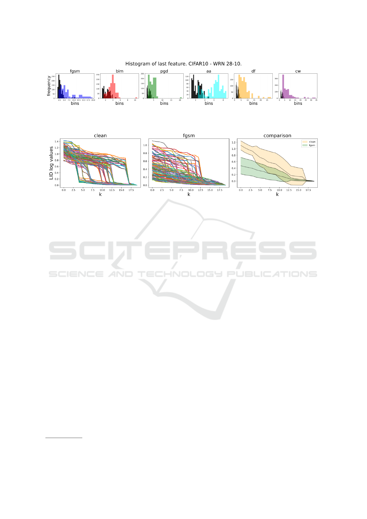
Figure 1: Visualization of the LID features from the clean set of samples (black) and different adversarial attacks of 100

samples. The network is WRN 28-10 trained on CIFAR10and LID is evaluated on the feature map after the last ReLU

activation.

Figure 2: Visualization of the LID features from the clean and FGSM set of 100 samples over each k. The network is WRN

28-10 trained on CIFAR10. The feature values for the nearest neighbors (low values on the x-axis) are signiﬁcantly higher

for the clean dataset. The plot on the right illustrates mean and standard deviation of the two sets of proﬁles.

4 EXPERIMENTS

To validate our proposed multiLID, we conduct

extensive experiments on CIFAR10, CIFAR100,

and ImageNet. We train two different models, a

wide-resnet (WRN 28-10) (Zagoruyko and Ko-

modakis, 2017; Wu et al., 2021) and a VGG-16

model (Simonyan and Zisserman, 2015) on the

different datasets. While we use test samples from

the original datasets as clean samples, we generate

adversarial samples using a variety of adversarial

attacks. From clean and adversarial data, we extract

the feature maps for different layers, at the output

of the ReLU activations. We use a random subset of

2000 samples of this data for each attack method and

extract the multiLID features from the feature maps.

From this random subset we take a train-test split of

80:20, i.e. we have a training set of 3200 samples

(1600 clean, 1600 attacked images) and a balanced

test set of 400 images for each attack. This setting

is common practice as used in (Ma et al., 2018; Lee

et al., 2018; Lorenz et al., 2022). All experiments

were conducted on 3 Nvidia A100 40GB GPUs

for ImageNet and 3 Nvidia Titan with 12GB for

CIFAR10 and CIFAR100.

Datasets. Many of the adversarial training methods

ranked on Robustbench

are based on the WRN

https://robustbench.github.io

28-10 (Zagoruyko and Komodakis, 2017; Wu et al.,

2021) architecture. Therefore, we also conduct our

evaluation on a baseline WRN 28-10 and train it with

clean examples.

CIFAR10: The CIFAR10 WRN 28-10 reaches a test

accuracy of 96% and the VGG-16 model reaches

72% top-1 accuracy (Lorenz et al., 2022) on the test

set. We then apply the different attacks on the test set.

CIFAR100: The procedure is equal to CI-

FAR10 dataset. We report a test-accuracy for

WRN 28-10 of 83% (VGG-16 reaches 81%) (Lorenz

et al., 2022) .

ImageNet: The PyTorch library provides a pre-trained

WRN 50-2 (Zagoruyko and Komodakis, 2017) for

ImageNet. As test set, we use the ofﬁcial validation

set from ImageNet and reach a validation accuracy of

80%.

Attack Methods. We generate test data from six

most commonly used adversarial attacks: FGSM,

BIM, PGD(-L

∞

), CW(-L

), DF(-L

) and AA, as

explained in section 2.1. For FGSM, BIM, PGD(-

∞

), and AA, we use the commonly employed

perturbation size of ε = 8/255, DF is limited to 20

iterations and CW to 1000 iterations.

Layer Feature Selection per Architecture. Fol-

lowing eq. (4), for the WRN 28-10 and WRN 50-2,

we focus on the ReLU activation layers, whereas

Unfolding Local Growth Rate Estimates for (Almost) Perfect Adversarial Detection

in each residual block, we take the last one. This

results in 13 activations layer for WRN 28-10 and 17

for WRN 50-2 to compute multiLID representations.

This is different from the setting proposed in (Yang

et al., 2021), who propose to use the outputs of the

three convolutional blocks. In (Ma et al., 2018) only

simpler network architectures have been considered

and the feature maps at the output of every layer

are considered to compute LID. For the VGG-16

architecture, according to (Harder et al., 2021), we

take the features of all activation layers, which are

again 13 layers in total.

Minibatch Size in LID Estimation. As motivated

in (Ma et al., 2018), we estimate the multiLID values

using a default minibatch size |B| of 100 with k se-

lected as of 20% of mini batch size (Ma et al., 2018).

As discussed above and theoretically argued before

in (Amsaleg et al., 2015) the MLE estimator of LID

suffers on such small samples, yet, already provides

reasonable results when used for adversarial detec-

tion (Ma et al., 2018). Our proposed multiLID can

perform very well in this computationally affordable

setting across all datasets.

4.1 Results

In this section, we report our ﬁnal results of our multi

LID method and compare it to competing methods.

In table 1, we compare the results of the original LID

(Ma et al., 2018) to the results of our proposed mul-

tiLID method for both model types, the wide-resnets

and VGG-16 models on the three datasets CIFAR10,

CIFAR100, and ImageNet. For LID and the proposed

multiLID, we extract features from exactly the same

layers in the network to facilitate direct comparison.

While LID already achieves overall good results the

proposed multiLID can even perfectly discriminate

between benign and adversarial images on these data

in terms of AUC as well as F1 score.

In table 2, we further compare the AUC and F1

score, for CIFAR10 trained on WRN 28-10 to a set of

most widely used adversarial defense methods. First,

we list the results from (Yang et al., 2021) for the de-

fenses kernel density (KD), LID and MD as baselines.

According to (Yang et al., 2021), KD does not show

strong results across the attacks, LID and MD yield a

better average performance in their setting. For com-

pleteness, we also report the results CD-VAE (Yang

et al., 2021) by showing R(x) (which is the recon-

struction of a sample x through a β variational auto en-

coder (β-VAE)). Encoding in such a well-conditioned

latent space can help adversarial detection, yet is also

time consuming and requires task speciﬁc training of

the β-VAE.

Our results, when reproducing LID on the same

network layers as (Yang et al., 2021), are reported in

the second block of table 2. While we can not exactly

reproduce the numbers from (Yang et al., 2021), the

resulting AUC and F1-scores are in the same order of

magnitude and slightly better in some cases. In this

setting, LID performs slightly worse than the compet-

ing methods MD and Spectral-BB and Spectral-WB

(Harder et al., 2021).

We ablate on our different changes towards the

full multiLID in the third block. When replacing

LID by the unfolded features as in eq. (9) we already

achieve results above 98% F1 score in all settings.

Defending against BIM is hardest. The next line ab-

lates on the employed feature maps. When replacing

the convolutional features used in (Yang et al., 2021)

by the last ReLU outputs in every block, we observe a

boost in performance even on the plain LID features.

Combining these two lead to almost perfect results.

Results for other datasets are in table 3. F1-scores

and AUC scores of consistently 100% can be reached

when classifying, on this feature basis, using a ran-

dom forest classiﬁer instead of the logistic regression.

We refer to this setting as multiLID in all other tables

including table 1.

5 ABLATION STUDY

In this section we give insights on the different fac-

tors affecting our approach. We investigate the impor-

tance of the activation maps the features are extracted

from as well as the number of multiLID features that

are needed to reach good classiﬁcation performance.

An ablation on the number of considered neighbors as

well as on the attack strength in terms of ε is provided

in the Appendix.

5.1 Impact of Non-Linear Classiﬁcation

In this section, we compare the methods from the last

two lines of table 2 in more detail and for all three

datasets. The results are reported in table 1. While

the simple logistic regression (LR) classiﬁer already

achieves very high AUC and F1 scores on multiLID

for all attacks and datasets, random forest (RF) can

further push the performance to even 100%.

Assumption of CD-VAE LID layers taken

from https://github.com/kai-wen-yang/CD-VAE/

blob/a33b5070d5d936396d51c8c2e7dedd62351ee5b2/

detection/models/wide resnet.py#L86.

VISAPP 2023 - 18th International Conference on Computer Vision Theory and Applications

Table 1: Results. Comparison of the original LID method with our proposed multiLID on different datasets. We report the

AUC and F1 score as mean and variance over three evaluations with randomly drawn test samples.

Attacks

CIFAR10 CIFAR100 ImageNet

WRN 28-10 VGG16 WRN 28-10 VGG16 WRN 50-2

auc f1 auc f1 auc f1 auc f1 auc f1

original LID (Ma et al., 2018)

FGSM 99.5±0.2 97.3±7.0 90.1±13.4 83.2±13.9 100.0±0.0 99.6±0.0 83.6±11.7 75.1±21.3 89.1±4.4 81.6±7.8

BIM 96.9±1.5 90.5±4.2 92.8±2.1 86.5±3.3 98.2±0.0 92.2±0.0 84.8±10.0 75.6±11.1 100.0±0.0 98.9±1.0

PGD 99.1±0.3 95.3±1.8 97.5±0.0 94.6±0.5 98.0±0.0 93.5±0.0 91.8±0.8 83.9±0.4 100.0±0.0 100.0±0.0

AA 96.7±0.2 89.4±3.4 90.0±1.3 81.6±1.8 99.2±0.1 96.5±0.4 86.8±9.8 78.6±2.3 100.0±0.0 99.8±0.1

DF 94.7±31.9 88.7±55.4 87.3±4.2 77.2±4.6 60.7±0.0 56.4±0.0 60.5±2.8 56.1±1.8 60.3±2.2 56.5±2.9

CW 91.2±63.6 83.9±54.5 85.2±1.7 75.3±3.5 56.3±0.1 52.5±2.6 66.0±6.1 61.0±0.9 62.0±0.5 59.0±2.0

multiLID + improved layer setting + RF or short: multiLID (ours)

FGSM 100.0±0.0 100.0±0.0 100.0±0.0 100.0±0.0 100.0±0.0 100.0±0.0 100.0±0.0 100.0±0.0 100.0±0.0 100.0±0.0

BIM 100.0±0.0 100.0±0.0 100.0±0.0 100.0±0.0 100.0±0.0 100.0±0.0 100.0±0.0 100.0±0.0 100.0±0.0 100.0±0.0

PGD 100.0±0.0 100.0±0.0 100.0±0.0 100.0±0.0 100.0±0.0 100.0±0.0 100.0±0.0 100.0±0.0 100.0±0.0 100.0±0.0

AA 100.0±0.0 100.0±0.0 100.0±0.0 100.0±0.0 100.0±0.0 100.0±0.0 100.0±0.0 100.0±0.0 100.0±0.0 100.0±0.0

DF 100.0±0.0 100.0±0.0 100.0±0.0 100.0±0.0 100.0±0.0 100.0±0.0 100.0±0.0 100.0±0.0 100.0±0.0 100.0±0.0

CW 100.0±0.0 100.0±0.0 100.0±0.0 100.0±0.0 100.0±0.0 100.0±0.0 100.0±0.0 100.0±0.0 100.0±0.0 100.0±0.0

Table 2: Comparison of multiLID with the state-of-the-art on CIFAR10.

CIFAR10 on WRN 28-10

Defenses

FGSM BIM PGD CW

TNR AUC TNR AUC TNR AUC TNR AUC

Results reported by (Yang et al., 2021)

KD 42.38 85.74 74.54 94.82 73.12 94.59 73.33 94.75

KD (R(x)) 57.10 89.69 96.79 99.27 96.56 99.30 94.67 98.73

LID 69.05 93.60 77.73 95.20 71.52 93.19 74.98 94.32

LID (R(x)) 92.60 98.59 86.42 97.29 87.54 97.57 76.42 95.10

MD 94.91 98.69 88.33 97.66 77.23 95.38 86.30 97.36

MD (R(x)) 99.68 99.36 98.92 99.74 99.13 99.79 98.94 99.68

Competing Methods

MD (Lee et al., 2018) 97.37 99.34 98.16 99.61 97.37 99.66 91.58 96.54

Spectral-BB (Harder et al., 2021) 95.79 99.87 92.63 99.83 92.11 99.29 53.68 63.23

Spectral-WB (Harder et al., 2021) 99.47 100.00 96.32 99.99 95.79 99.97 84.47 96.89

LID, settings from (Yang et al., 2021) 79.47 90.29 75.79 77.79 73.68 73.79 77.11 81.20

Ours

multiLID, settings from (Yang et al., 2021) 100.00 100.00 99.47 98.68 100.00 100.00 100.00 100.00

LID, improved layer setting 97.37 99.81 88.42 95.73 86.58 93.02 94.74 98.81

multiLID + improved layer setting 100.00 100.00 100.00 100.00 100.00 100.00 99.61 100.00

multiLID + improved layer setting + RF 100.00 100.00 100.00 100.00 100.00 100.00 100.00 100.00

Table 3: Results of using multiLID. Comparison of Logistic Regression and Random Forest classiﬁer on different datasets.

Comparison to table 1 which uses logistic regression (LR). The minibatch size is |B| = 100 and the number of neighbors

k = 20 according to section 4.

Attacks

CIFAR10 CIFAR100 ImageNet

WRN 28-10 VGG16 WRN 28-10 VGG16 WRN 50-2

auc f1 auc f1 auc f1 auc f1 auc f1

multiLID + LR

FGSM 100.0±0.0 100.0±0.0 100.0±0.0 100.0±0.0 100.0±0.0 100.0±0.0 100.0±0.0 100.0±0.0 100.0±0.0 100.0±0.0

BIM 100.0±0.0 100.0±0.0 100.0±0.0 100.0±0.0 100.0±0.0 100.0±0.0 100.0±0.0 100.0±0.0 100.0±0.0 100.0±0.0

PGD 100.0±0.0 100.0±0.0 100.0±0.0 100.0±0.0 100.0±0.0 100.0±0.0 100.0±0.0 100.0±0.0 100.0±0.0 100.0±0.0

AA 100.0±0.0 100.0±0.0 100.0±0.0 100.0±0.0 100.0±0.0 100.0±0.0 100.0±0.0 100.0±0.0 100.0±0.0 100.0±0.0

DF 100.0±0.0 99.9±0.0 100.0±0.0 99.9±0.0 100.0±0.0 98.5±0.0 100.0±0.0 99.9±0.0 99.8±0.0 98.3±0.6

CW 100.0±0.0 99.9±0.0 100.0±0.0 100.0±0.0 99.9±0.0 98.0±0.2 100.0±0.0 99.9±0.0 99.9±0.0 99.1±0.2

multiLID + RF (ours)

FGSM 100.0±0.0 100.0±0.0 100.0±0.0 100.0±0.0 100.0±0.0 100.0±0.0 100.0±0.0 100.0±0.0 100.0±0.0 100.0±0.0

BIM 100.0±0.0 100.0±0.0 100.0±0.0 100.0±0.0 100.0±0.0 100.0±0.0 100.0±0.0 100.0±0.0 100.0±0.0 100.0±0.0

PGD 100.0±0.0 100.0±0.0 100.0±0.0 100.0±0.0 100.0±0.0 100.0±0.0 100.0±0.0 100.0±0.0 100.0±0.0 100.0±0.0

AA 100.0±0.0 100.0±0.0 100.0±0.0 100.0±0.0 100.0±0.0 100.0±0.0 100.0±0.0 100.0±0.0 100.0±0.0 100.0±0.0

DF 100.0±0.0 100.0±0.0 100.0±0.0 100.0±0.0 100.0±0.0 100.0±0.0 100.0±0.0 100.0±0.0 100.0±0.0 100.0±0.0

CW 100.0±0.0 100.0±0.0 100.0±0.0 100.0±0.0 100.0±0.0 100.0±0.0 100.0±0.0 100.0±0.0 100.0±0.0 100.0±0.0

Unfolding Local Growth Rate Estimates for (Almost) Perfect Adversarial Detection

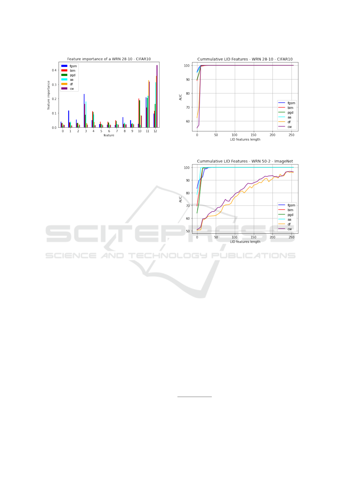
Figure 3: Feature importance. Increasing order according

to the activation function layers (feature) from WRN 28-

10 trained on CIFAR10. The most relevant features are in

the last ReLU layers.

5.2 Feature Importance

The feature importance (variable importance) of the

random forest describes the relevant features for the

detection. In ﬁg. 3, we plot the feature importance for

the aggregated LID features of WRN 28-10 trained

on a CIFAR10 dataset. The feature importance repre-

sents the importance of the selected ReLU layers (see

(Lee et al., 2018)) in increasing order. The last fea-

tures/layers shows higher importance. For the attack

FGSM the 3rd and last feature can be very relevant.

5.3 Investigation of the multiLID

Features

Following the eq. (2), all neighbors k are used for the

classiﬁcation. This time, we investigate the perfor-

mance of the binary classiﬁer logistic regression over

the full multiLID features. For example, in ﬁg. 3 we

consider 13 layers and the aggregated ID features for

each. Thus, the number of multiLID features per sam-

ple can be calculated as #layers × k which yields 260

features for k = 20. In ﬁg. 4, we visualize the AUC ac-

cording to the length of the LID feature vectors, when

successively more features are used according to their

random forest feature importance. On ImageNet, it

can be seen that DF and CW need the full length of

these LID feature vectors to achieve the highest AUC

scores. The observation, that the attacks DF and CW

are more effectively are also reported in (Lorenz et al.,

2022). Using a non-linear classiﬁer on these very dis-

criminant features, we can even achieve perfect F1

scores (see section 5.1).

(a) Cummulative of all attacks on CIFAR10.

(b) Cummulative of all attacks on ImageNet.

Figure 4: Cummulative features used for the LR classiﬁer.

The x-axis describes the length of the used feature vectors.

The y-axis reports the AUC reached by using the most im-

portant features out of the full vector, sorted by RF feature

importance.

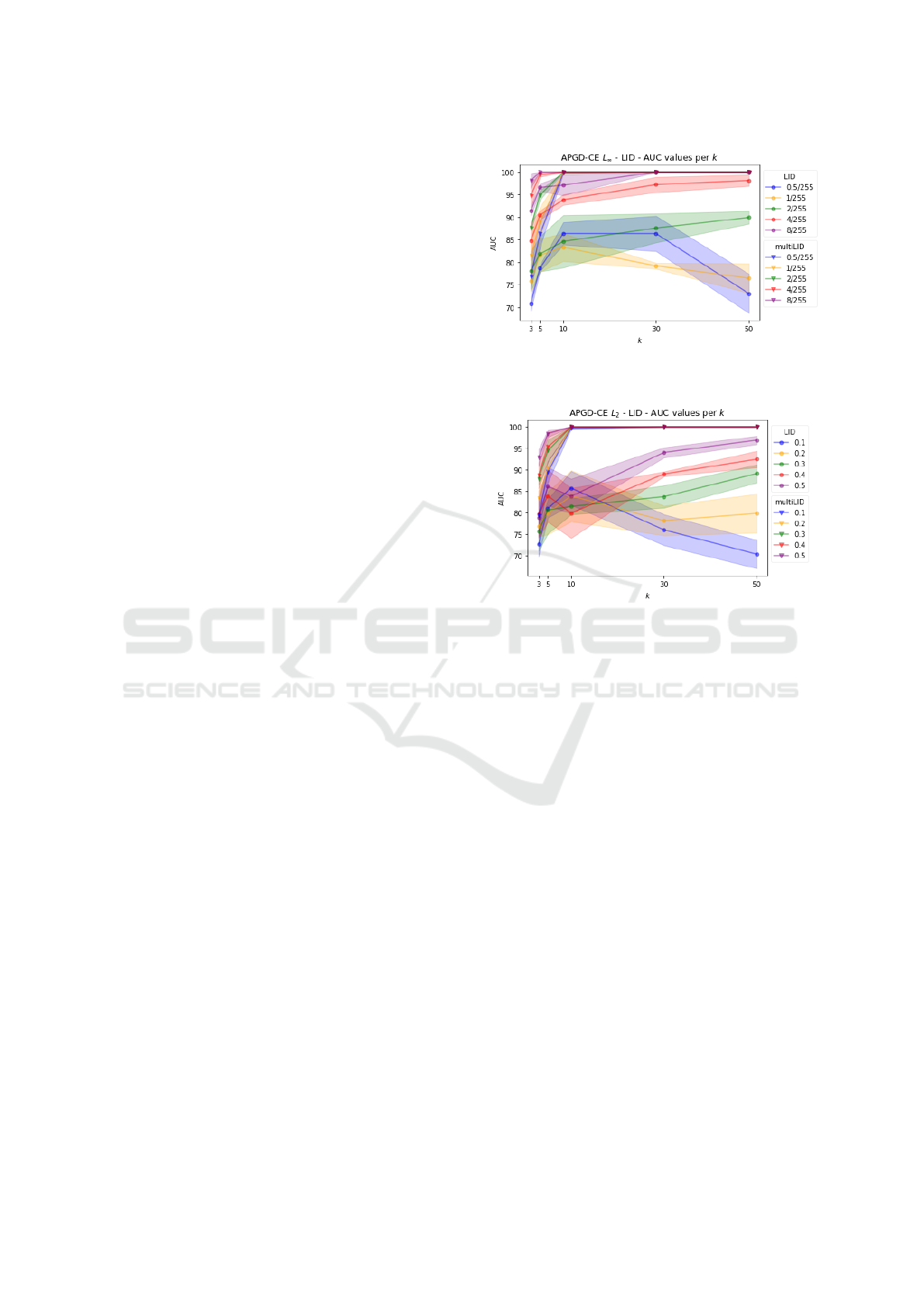
5.4 Impact of the Number of Neighbors

We train the LID with the APGD-CE attack from the

AutoAttack benchmark with different epsilons (L

∞

and L

). In ﬁg. 5, we compare RF and LR on different

norms. Random Forest succeeds on all epsilons sizes

on both norms. On smaller perturbation sizes the LR

classiﬁer AUC score fall. On the optimal perturbation

size (L

∞

: ε = 8/255 and L

: ε = 0.5) the LR shows

its best AUC scores. The RF classiﬁer gives us out-

standing results over the LR. Moreover, to save com-

putation time, k = 3 neighbors would be enough for

high accuracy.

Perturbed images would round the adversarial changes

to the next of 256 available bins in commonly used 8-bit per

channel image encodings.

VISAPP 2023 - 18th International Conference on Computer Vision Theory and Applications

6 CONCLUSION

In this paper, we revisit the MLE estimate of the

local intrinsic dimensionality which has been used in

previous works on adversarial detection. An analysis

of the extracted LID features and their theoretical

properties allows us to redeﬁne an LID-based feature

using unfolded local growth rate estimates that are

signiﬁcantly more discriminative than the aggregated

LID measure.

Limitations. While our method allows to achieve al-

most perfect to perfect results in the considered test

scenario and for the given datasets, we do not claim

to have solved the actual problem. We use the evalu-

ation setting as proposed in previous works (e.g.(Ma

et al., 2018)) where each attack method is evaluated

separately and with constant attack parameters. For a

deployment in real-world scenarios, the robustness of

a detector under potential disguise mechanisms needs

to be veriﬁed. An extended study on the transfer-

ability of our method from one attack to the other

can be found in the supplementary material. It shows

ﬁrst promising resulting in this respect but also leaves

room for further improvement.

REFERENCES

Amsaleg, L., Bailey, J., Barbe, A., Erfani, S. M., Furon, T.,

Houle, M. E., Radovanovi

c, M., and Nguyen, X. V.

(2021). High intrinsic dimensionality facilitates ad-

versarial attack: Theoretical evidence. IEEE Transac-

tions on Information Forensics and Security, 16:854–

865.

Amsaleg, L., Chelly, O., Furon, T., Girard, S., Houle, M. E.,

Kawarabayashi, K.-i., and Nett, M. (2015). Estimat-

ing local intrinsic dimensionality. In SIGKDD, page

29–38, New York, NY, USA. Association for Comput-

ing Machinery.

Andriushchenko, M., Croce, F., Flammarion, N., and Hein,

M. (2020). Square attack: a query-efﬁcient black-box

adversarial attack via random search. In ECCV.

Carlini, N. and Wagner, D. (2017a). Magnet and ”efﬁcient

defenses against adversarial attacks” are not robust to

adversarial examples.

Carlini, N. and Wagner, D. A. (2017b). Towards evaluating

the robustness of neural networks. IEEE Symposium

on Security and Privacy (SP), pages 39–57.

Croce, F. and Hein, M. (2020a). Minimally distorted adver-

sarial examples with a fast adaptive boundary attack.

In ICML.

Croce, F. and Hein, M. (2020b). Reliable evaluation of

adversarial robustness with an ensemble of diverse

parameter-free attacks. In ICML.

Evtimov, I., Eykholt, K., Fernandes, E., Kohno, T., Li, B.,

Prakash, A., Rahmati, A., and Song, D. (2017). Ro-

bust physical-world attacks on deep learning models.

CVPR.

Feinman, R., Curtin, R. R., Shintre, S., and Gardner, A. B.

(2017). Detecting adversarial samples from artifacts.

ICML, abs/1703.00410.

Goodfellow, I., Shlens, J., and Szegedy, C. (2015). Ex-

plaining and harnessing adversarial examples. ICLR,

abs/1412.6572.

Harder, P., Pfreundt, F.-J., Keuper, M., and Keuper, J.

(2021). Spectraldefense: Detecting adversarial attacks

on cnns in the fourier domain. In IJCNN.

Houle, M. E. (2017a). Local intrinsic dimensionality i: An

extreme-value-theoretic foundation for similarity ap-

plications. In Beecks, C., Borutta, F., Kr

oger, P., and

Seidl, T., editors, Similarity Search and Applications,

pages 64–79, Cham. Springer International Publish-

ing.

Houle, M. E. (2017b). Local intrinsic dimensionality ii:

Multivariate analysis and distributional support. In

Beecks, C., Borutta, F., Kr

oger, P., and Seidl, T., edi-

tors, Similarity Search and Applications, pages 80–95,

Cham. Springer International Publishing.

Houle, M. E., Kashima, H., and Nett, M. (2012). Gener-

alized expansion dimension. In IEEE 12th Interna-

tional Conference on Data Mining Workshops, pages

587–594.

Karger, D. R. and Ruhl, M. (2002). Finding nearest neigh-

bors in growth-restricted metrics. In Proceedings of

the Thiry-Fourth Annual ACM Symposium on Theory

of Computing, page 741–750, New York, NY, USA.

Association for Computing Machinery.

Kurakin, A., Goodfellow, I., and Bengio, S. (2017). Adver-

sarial examples in the physical world. In ICLR.

Lee, K., Lee, K., Lee, H., and Shin, J. (2018). A simple uni-

ﬁed framework for detecting out-of-distribution sam-

ples and adversarial attacks. In NeurIPS.

Lorenz, P., Harder, P., Straßel, D., Keuper, M., and Keu-

per, J. (2021). Detecting autoattack perturbations in

the frequency domain. In ICML 2021 Workshop on

Adversarial Machine Learning.

Lorenz, P., Strassel, D., Keuper, M., and Keuper, J. (2022).

Is robustbench/autoattack a suitable benchmark for

adversarial robustness? In The AAAI-22 Workshop

on Adversarial Machine Learning and Beyond.

Ma, X., Li, B., Wang, Y., Erfani, S., Wijewickrema, S.,

Houle, M., Schoenebeck, G., Song, D., and Bailey,

J. (2018). Characterizing adversarial subspaces using

local intrinsic dimensionality. ICLR, abs/1801.02613.

Madry, A., Makelov, A., Schmidt, L., Tsipras, D., and

Vladu, A. (2018). Towards deep learning models re-

sistant to adversarial attacks. ICLR, abs/1706.06083.

Moosavi-Dezfooli, S.-M., Fawzi, A., and Frossard, P.

(2016). Deepfool: A simple and accurate method to

fool deep neural networks. CVPR, pages 2574–2582.

Rice, L., Wong, E., and Kolter, Z. (2020). Overﬁtting in

adversarially robust deep learning. In ICML, pages

8093–8104. PMLR.

Sharif, M., Bhagavatula, S., Bauer, L., and Reiter, M. K.

(2019). A general framework for adversarial examples

Unfolding Local Growth Rate Estimates for (Almost) Perfect Adversarial Detection

with objectives. ACM Transactions on Privacy and

Security, 22(3):1–30.

Simonyan, K. and Zisserman, A. (2015). Very deep con-

volutional networks for large-scale image recognition.

ICLR, abs/1409.1556.

Szegedy, C., Zaremba, W., Sutskever, I., Bruna, J., Erhan,

D., Goodfellow, I., and Fergus, R. (2014). Intriguing

properties of neural networks. ICLR.

Wong, E., Rice, L., and Kolter, J. Z. (2020). Fast is better

than free: Revisiting adversarial training. In ICLR.

Wu, B., Chen, J., Cai, D., He, X., and Gu, Q. (2021). Do

wider neural networks really help adversarial robust-

ness? In Beygelzimer, A., Dauphin, Y., Liang, P., and

Vaughan, J. W., editors, NeurIPS.

Yang, K., Zhou, T., Zhang, Y., Tian, X., and Tao, D. (2021).

Class-disentanglement and applications in adversarial

detection and defense. In Beygelzimer, A., Dauphin,

Y., Liang, P., and Vaughan, J. W., editors, NeurIPS.

Zagoruyko, S. and Komodakis, N. (2017). Wide residual

networks. In BMVC.

APPENDIX

A. Impact of the Number of Neighbors

and Attack Strength ε

We train LID and multiLID with the APGD-CE attack

from the AutoAttack benchmark for different pertur-

bation magnitudes, i.e. using different epsilons (L

∞

and L

). On smaller perturbation sizes the logistic

regression (LR) classiﬁer AUC scores are dropping,

which is to be expected. On the most commonly used

perturbation sizes (L

∞

: ε = 8/255 and L

: ε = 0.5)

LID shows its best AUC scores. The multiLID classi-

ﬁer provides superior results over LID in all cases.

Moreover, to save computation time for multiLID,

k = 10 neighbors would be enough for high accuracy

adversarial detection.

B. Attack Transferability

In this section, we evaluate the attack transferability

of our models, for LID in table 4 and multiLID in ta-

ble 4. In case of real world applications, the attack

methods might be unknown and thus it is a desired

feature that a detector trained on one attack method

performs well for a different attack. We evaluate in

both directions. The random forest (RF) classiﬁer

shows signiﬁcantly higher transferability on both LID

and multiLID. The attack tuples (pgd ↔ bim), (pgd

↔ aa), (aa ↔ bim), and (df ↔ cw) yield very high

bidirectional attack transferability. However, the ex-

periments also show that not all combinations can be

(a) The attack APGD-CE L

∞

evaluated on different epsilons

and neighbors.

(b) The attack APGD-CE L

evaluated on different epsilons

and neighbors.

Figure 5: Ablation study of LID and multiLID detection

rates by using different k on the APGD-CE (L

, L

∞

) attack

and different epsilon sizes.

transferred successfully, e.g. (fgsm ↔ cw) in Ima-

geNet. This leaves room for further research.

VISAPP 2023 - 18th International Conference on Computer Vision Theory and Applications

Table 4: Attack transfer LID. Rows with the target µ give the average transfer rates from one attack to all others. RF shows

higher accuracy (acc) for the attack transfer.

LID

Attacks

CIFAR10 CIFAR100 ImageNet

WRN 28-10 VGG16 WRN 28-10 VGG16 WRN 50-2

from to auc acc auc acc auc acc auc acc auc acc

logistic regression

fgsm bim 50.0±0.0 50.0±0.0 69.4±2.9 52.8±2.6 50.0±0.0 50.0±0.0 72.7±5.8 53.7±4.3 74.0±8.0 56.7±6.3

fgsm pgd 50.0±0.0 50.0±0.0 67.9±3.9 52.0±1.8 50.0±0.0 50.0±0.0 75.0±6.4 53.7±4.0 78.3±5.8 57.4±6.5

fgsm aa 50.1±0.1 50.0±0.0 70.4±10.6 52.0±1.8 50.0±0.0 50.0±0.0 67.2±3.7 50.2±1.1 72.6±11.7 60.9±9.1

fgsm df 50.0±0.0 50.0±0.0 58.0±0.9 51.9±1.7 50.0±0.0 50.0±0.0 53.0±1.0 51.5±1.4 49.6±0.9 50.5±0.5

fgsm cw 50.0±0.0 50.0±0.0 57.1±1.2 51.5±1.4 50.0±0.0 50.0±0.0 55.5±3.1 53.2±3.8 49.5±0.9 50.6±0.7

fgsm µ 50.0±0.0 50.0±0.0 64.5±7.5 52.0±1.7 50.0±0.0 50.0±0.0 64.7±10.0 52.4±3.1 64.8±14.3 55.2±6.4

bim fgsm 60.1±15.1 55.1±8.8 66.8±5.6 49.9±0.2 50.0±0.0 50.0±0.0 71.4±2.1 60.5±6.2 50.0±0.0 50.0±0.0

bim pgd 52.7±0.4 50.0±0.0 74.9±8.0 50.0±0.0 50.0±0.0 50.0±0.0 86.0±3.7 66.1±10.7 50.0±0.0 50.0±0.0

bim aa 51.4±1.2 50.0±0.0 76.1±9.8 50.0±0.0 50.0±0.0 50.0±0.0 77.5±1.6 59.7±9.7 50.5±0.8 50.0±0.0

bim df 52.6±0.4 50.0±0.0 55.0±3.2 50.0±0.0 50.0±0.0 50.0±0.0 52.1±0.8 50.4±0.8 50.0±0.0 50.0±0.0

bim cw 52.1±0.0 50.0±0.0 55.7±2.5 50.0±0.0 50.0±0.0 50.0±0.0 61.0±2.5 56.8±4.4 50.0±0.0 50.0±0.0

bim µ 53.8±6.6 51.0±3.9 65.7±10.8 50.0±0.1 50.0±0.0 50.0±0.0 69.6±12.5 58.7±8.2 50.1±0.4 50.0±0.0

pgd fgsm 57.6±10.6 52.8±4.8 71.4±6.6 50.4±0.7 50.0±0.0 50.0±0.0 71.2±1.3 62.3±2.9 50.0±0.0 50.0±0.0

pgd bim 53.3±2.0 50.0±0.0 78.2±7.7 50.5±0.8 50.0±0.0 50.0±0.0 82.7±2.9 72.2±4.6 50.0±0.0 50.0±0.0

pgd aa 53.0±3.4 50.0±0.0 76.8±6.2 49.7±0.5 50.8±1.3 50.1±0.1 77.6±1.3 72.5±1.8 50.0±0.0 50.0±0.0

pgd df 52.5±1.5 50.0±0.0 52.9±2.1 50.5±0.8 50.0±0.0 50.0±0.0 51.4±0.6 51.8±2.0 50.0±0.0 50.0±0.0

pgd cw 52.0±0.9 50.0±0.0 54.3±1.6 50.5±0.8 50.0±0.0 50.0±0.0 61.7±2.4 57.7±1.6 50.0±0.0 50.0±0.0

pgd µ 53.7±4.8 50.5±2.1 66.7±12.2 50.3±0.7 50.2±0.6 50.0±0.0 68.9±11.7 63.3±8.7 50.0±0.0 50.0±0.0

aa fgsm 51.0±0.9 50.1±0.2 59.6±3.3 49.0±1.0 53.5±2.3 50.4±0.4 52.4±2.8 50.0±0.0 50.0±0.0 50.0±0.0

aa bim 50.4±0.6 50.0±0.0 61.4±3.8 47.7±2.4 54.6±2.6 50.2±0.3 52.6±2.2 50.0±0.0 50.0±0.0 50.0±0.0

aa pgd 50.4±0.6 50.0±0.0 59.9±3.2 47.8±1.9 54.6±2.6 50.2±0.3 52.0±2.4 50.0±0.0 50.0±0.0 50.0±0.0

aa df 50.2±0.3 50.0±0.0 58.3±5.0 49.6±0.4 52.4±2.0 50.0±0.0 50.5±0.7 50.0±0.0 50.0±0.0 50.0±0.0

aa cw 50.2±0.3 50.0±0.0 56.8±3.4 49.6±0.4 52.0±1.4 49.9±0.2 50.5±0.8 50.0±0.0 50.0±0.0 50.0±0.0

aa µ 50.4±0.6 50.0±0.1 59.2±3.6 48.7±1.5 53.4±2.2 50.1±0.3 51.6±1.9 50.0±0.0 50.0±0.0 50.0±0.0

df fgsm 70.6±14.1 52.2±3.8 61.0±13.6 52.2±4.8 98.3±0.0 52.1±0.0 63.7±9.1 53.0±2.1 52.2±2.5 50.5±0.5

df bim 75.9±14.7 50.2±0.4 61.6±7.7 54.6±4.9 82.0±0.0 51.1±0.4 65.4±3.1 51.3±1.4 1.0±1.0 49.3±0.5

df pgd 75.3±14.1 50.2±0.4 58.2±6.6 54.9±4.7 73.6±3.2 50.4±0.2 69.4±5.2 53.3±4.1 0.3±0.4 49.3±0.5

df aa 71.4±22.9 50.2±0.4 69.3±12.9 56.6±5.7 81.6±3.5 58.5±4.4 59.1±1.0 45.7±0.2 0.0±0.0 48.0±1.5

df cw 68.3±1.0 50.2±0.4 68.7±6.2 57.9±7.0 55.0±0.2 50.8±0.4 57.6±2.1 51.6±0.9 61.6±2.0 50.5±1.0

df µ 72.3±13.1 50.6±1.7 63.8±9.6 55.2±5.1 78.1±14.7 52.6±3.5 63.0±6.1 51.0±3.4 23.0±28.8 49.5±1.2

cw fgsm 67.9±15.3 58.8±15.2 62.5±10.9 53.9±6.3 89.1±0.8 81.9±2.0 57.6±2.5 50.4±0.5 53.1±2.7 50.0±0.8

cw bim 74.5±15.3 53.6±6.3 69.0±3.2 59.3±8.1 89.7±0.9 78.8±1.9 74.1±5.6 54.9±6.8 1.2±1.2 48.7±0.7

cw pgd 74.3±15.7 53.5±6.1 64.1±2.7 57.8±6.8 93.6±3.1 84.1±3.7 81.0±2.9 56.3±8.7 0.3±0.6 48.7±0.7

cw aa 69.9±22.5 53.4±6.0 75.1±11.8 59.2±9.7 85.8±3.2 61.0±9.9 67.1±3.1 52.9±3.1 0.0±0.0 45.8±4.0

cw df 68.9±5.7 52.5±4.3 71.9±8.8 61.3±12.8 52.2±0.3 52.6±0.3 53.7±1.5 50.9±1.2 60.0±2.8 50.3±1.0

cw µ 71.1±13.7 54.4±7.5 68.5±8.6 58.3±8.1 82.1±15.8 71.7±13.6 66.7±10.9 53.1±4.9 22.9±28.6 48.7±2.3

random forest

fgsm bim 74.1±14.5 57.8±8.3 89.5±2.2 78.0±4.8 83.3±0.0 69.5±0.0 73.9±3.4 68.4±3.6 63.4±10.0 55.5±5.4

fgsm pgd 75.3±15.1 58.8±9.2 86.3±3.4 72.5±5.5 82.8±0.2 68.3±0.6 76.9±2.3 69.9±2.6 61.5±6.9 53.6±2.8

fgsm aa 83.5±4.5 62.0±9.5 84.4±1.0 74.4±0.9 83.4±7.6 71.5±5.8 73.5±3.0 66.5±4.9 35.0±11.5 38.1±5.6

fgsm df 77.6±17.9 59.1±8.7 83.1±1.3 71.5±5.0 53.9±0.0 53.0±0.0 56.8±3.2 54.6±1.6 51.9±1.2 49.8±1.0

fgsm cw 74.3±17.0 54.6±5.2 81.5±1.6 68.5±3.6 51.6±0.4 50.7±0.0 55.8±2.2 52.7±1.1 51.5±1.5 50.2±1.2

fgsm µ 77.0±12.9 58.5±7.5 85.0±3.4 73.0±4.9 71.0±15.7 62.6±9.4 67.4±9.8 62.4±8.0 52.6±12.2 49.4±7.0

bim fgsm 93.8±3.8 79.3±1.5 87.7±2.1 76.2±5.8 91.4±0.0 63.5±0.0 72.8±0.9 63.9±3.6 63.7±2.0 49.4±0.9

bim pgd 100.0±0.0 92.8±2.6 100.0±0.0 88.0±3.3 100.0±0.0 97.3±1.8 99.7±0.5 92.5±3.4 100.0±0.0 99.6±0.7

bim aa 92.3±6.7 87.0±10.4 94.0±1.2 89.1±4.5 88.8±4.9 74.5±2.6 85.5±5.9 76.9±7.8 99.0±1.5 97.9±1.5

bim df 99.9±0.2 79.5±10.3 99.4±0.6 72.8±3.4 98.4±0.0 51.6±0.0 88.0±20.1 57.1±0.5 78.4±21.2 51.5±2.5

bim cw 99.6±0.6 71.9±12.6 99.3±0.4 72.6±1.9 98.1±0.4 50.4±0.0 89.3±17.8 59.2±1.6 94.3±3.0 50.6±0.5

bim µ 97.1±4.6 82.1±10.5 95.3±4.9 67.4±18.0 96.1±5.0 79.7±8.3 87.1±13.7 69.9±14.1 87.1±16.6 69.8±24.5

pgd fgsm 92.4±4.2 77.3±1.9 88.3±1.0 77.7±1.8 92.8±2.4 63.6±1.8 72.2±3.3 59.9±2.0 60.2±5.3 50.1±0.4

pgd bim 100.0±0.0 94.0±2.2 100.0±0.0 95.2±3.0 99.8±0.4 92.4±0.4 98.8±2.0 87.7±1.6 100.0±0.0 97.7±0.9

pgd aa 90.0±8.7 84.4±13.6 92.4±2.5 85.4±3.1 87.1±3.2 71.6±1.4 84.8±2.8 76.7±3.1 99.8±0.2 99.4±0.7

pgd df 99.3±1.2 81.9±9.9 99.4±0.5 70.7±5.1 92.4±1.1 52.7±0.6 79.7±17.8 56.7±2.4 79.9±23.3 51.0±1.7

pgd cw 99.6±0.7 74.9±13.8 99.4±0.5 73.2±3.3 93.6±1.4 52.1±0.0 81.3±16.5 59.6±2.1 96.1±2.1 50.3±0.5

pgd µ 96.5±5.6 83.6±11.3 95.9±5.0 80.4±9.7 93.1±4.5 66.5±15.4 83.4±13.0 68.2±12.6 87.2±18.3 69.7±24.4

aa fgsm 91.0±0.8 80.6±3.9 81.4±5.7 70.2±6.7 90.5±6.3 76.7±5.7 66.7±0.7 56.7±0.3 51.1±6.5 50.0±0.0

aa bim 88.1±10.3 72.8±13.1 87.7±4.3 79.6±3.5 92.7±2.2 85.7±1.0 78.0±2.1 67.4±3.3 81.3±1.8 68.2±1.3

aa pgd 86.7±11.8 69.9±12.3 82.9±3.8 74.2±2.3 94.0±2.5 86.5±1.1 81.1±3.5 70.9±4.5 91.0±2.4 81.4±2.5

aa df 79.6±17.2 61.1±2.2 81.8±2.4 69.4±0.2 53.1±2.2 50.6±1.3 50.0±1.8 46.5±2.3 49.5±1.0 50.0±0.0

aa cw 73.8±20.2 52.9±0.7 79.9±2.3 67.9±1.1 52.4±0.4 50.5±0.8 51.5±0.9 47.6±1.7 50.4±1.5 50.0±0.0

aa µ 83.8±13.3 67.5±12.2 82.7±4.3 72.3±5.3 76.5±20.3 70.0±17.0 65.5±13.5 57.8±10.6 64.7±18.6 59.9±13.3

df fgsm 91.9±4.0 83.9±7.1 83.9±2.7 72.9±4.6 77.2±0.4 67.5±0.9 59.5±5.9 54.6±5.8 56.9±2.4 52.0±1.2

df bim 100.0±0.0 87.8±7.7 98.9±1.8 87.8±3.7 100.0±0.0 72.0±1.7 92.8±12.5 71.6±7.7 100.0±0.0 55.3±2.6

df pgd 100.0±0.0 88.7±7.5 99.4±1.1 81.1±5.1 100.0±0.0 65.8±1.6 89.2±10.7 72.8±8.0 100.0±0.0 54.4±2.9

df aa 85.2±13.2 74.9±23.0 84.7±7.4 78.5±5.8 46.2±1.7 45.1±2.1 48.4±8.4 50.2±6.8 38.4±28.2 41.8±26.0

df cw 100.0±0.0 91.6±4.8 100.0±0.0 95.5±2.0 100.0±0.0 89.5±1.4 100.0±0.0 87.5±2.4 100.0±0.0 89.7±0.6

df µ 95.4±8.1 85.4±11.8 93.4±8.3 83.2±8.9 84.7±21.9 68.0±14.7 78.0±22.2 67.3±15.0 79.1±29.3 58.6±19.5

cw fgsm 86.1±13.0 75.1±21.8 84.5±1.2 76.8±2.8 66.2±1.0 62.0±1.1 57.8±4.2 55.0±2.3 52.8±2.3 54.4±1.4

cw bim 100.0±0.0 90.2±4.4 99.1±1.5 91.4±3.2 100.0±0.0 62.5±1.3 94.7±9.2 75.6±1.3 100.0±0.0 57.8±3.1

cw pgd 100.0±0.0 89.2±5.7 98.6±2.0 84.9±4.0 100.0±0.0 59.9±4.0 91.7±7.5 77.9±4.6 100.0±0.0 55.1±3.9

cw aa 83.7±14.4 77.1±19.8 84.9±8.1 75.2±10.2 48.9±4.8 47.6±4.4 55.8±8.7 58.9±7.4 34.2±34.4 37.0±27.9

cw df 100.0±0.0 96.5±3.6 100.0±0.0 98.2±1.5 100.0±0.0 95.3±0.8 100.0±0.0 86.5±4.1 100.0±0.0 84.4±1.4

cw µ 94.0±10.6 85.6±14.3 93.4±8.1 85.3±10.0 83.0±22.4 65.5±16.6 80.0±20.6 70.8±12.9 77.4±32.1 57.7±19.1

Unfolding Local Growth Rate Estimates for (Almost) Perfect Adversarial Detection

Table 5: Attack transfer multiLID. Rows with the target µ give the average transfer rates from one attack to all others. The

full multiLID with RF shows signiﬁcantly better acccuracy (acc) for the attack transfer.

multiLID

Attacks

CIFAR10 CIFAR100 ImageNet

WRN 28-10 VGG16 WRN 28-10 VGG16 WRN 50-2

from to auc acc auc acc auc acc auc acc auc acc

logistic regression

fgsm bim 92.8±0.6 50.0±0.0 82.4±5.8 50.0±0.0 90.9±0.5 50.0±0.0 79.3±0.7 50.0±0.0 70.1±8.3 50.0±0.0

fgsm pgd 96.1±0.4 50.0±0.0 76.8±7.0 50.0±0.0 94.5±1.4 50.0±0.0 78.9±4.4 50.0±0.0 63.6±13.0 50.0±0.0

fgsm aa 84.4±13.3 50.0±0.0 91.9±1.5 50.0±0.0 87.2±3.1 50.0±0.0 85.5±1.1 50.0±0.0 71.8±8.6 50.0±0.0

fgsm df 99.6±0.1 50.0±0.0 86.2±4.0 50.0±0.0 68.2±1.0 50.0±0.0 64.6±5.4 50.0±0.0 51.5±4.8 50.2±0.3

fgsm cw 99.8±0.1 50.0±0.0 85.0±4.4 50.0±0.0 62.9±0.6 50.0±0.0 63.2±5.3 50.0±0.0 52.5±5.1 50.0±0.0

fgsm µ 94.5±7.8 50.0±0.0 84.4±6.6 50.0±0.0 80.7±13.2 50.0±0.0 74.3±9.7 50.0±0.0 61.9±11.4 50.0±0.1

bim fgsm 96.7±1.5 50.0±0.0 84.9±2.4 50.0±0.0 87.1±1.0 50.0±0.0 76.0±1.5 50.0±0.0 50.7±4.2 50.0±0.0

bim pgd 97.0±0.1 50.0±0.0 82.7±7.1 50.0±0.0 95.3±0.3 50.0±0.0 87.1±1.6 50.9±1.6 99.9±0.1 50.0±0.0

bim aa 83.3±14.4 50.0±0.0 94.7±1.1 50.0±0.0 84.6±3.9 50.0±0.0 89.0±2.1 50.0±0.0 100.0±0.0 50.0±0.0

bim df 99.7±0.0 50.0±0.0 87.5±2.2 50.0±0.0 67.1±1.2 50.0±0.0 62.5±4.7 50.0±0.0 40.9±1.0 50.0±0.0

bim cw 99.8±0.0 50.0±0.0 86.2±2.7 50.0±0.0 63.9±1.0 50.0±0.0 63.1±5.7 50.0±0.0 40.7±0.9 50.0±0.0

bim µ 95.3±8.4 50.0±0.0 87.2±5.3 50.0±0.0 79.6±12.6 50.0±0.0 75.6±12.1 50.2±0.7 66.4±28.6 50.0±0.0

pgd fgsm 96.7±1.6 50.0±0.0 84.9±1.2 50.0±0.0 83.9±1.1 50.0±0.0 76.6±0.2 50.0±0.0 50.5±2.7 50.0±0.0

pgd bim 93.8±0.0 50.0±0.0 89.9±6.6 50.0±0.0 93.0±0.7 50.0±0.0 87.0±1.3 50.0±0.0 99.7±0.3 50.0±0.0

pgd aa 83.2±14.3 50.0±0.0 94.4±2.0 50.0±0.0 87.0±3.1 50.0±0.0 88.9±1.4 50.0±0.0 100.0±0.0 50.0±0.0

pgd df 99.7±0.0 50.0±0.0 86.5±3.2 50.0±0.0 63.4±2.1 50.0±0.0 62.0±4.0 50.0±0.0 40.8±1.0 50.0±0.0

pgd cw 99.8±0.0 50.0±0.0 85.0±3.3 50.0±0.0 61.1±1.9 50.0±0.0 64.8±1.3 50.0±0.0 40.5±1.3 50.0±0.0

pgd µ 94.7±8.4 50.0±0.0 88.1±4.9 50.0±0.0 77.7±13.5 50.0±0.0 75.8±11.5 50.0±0.0 66.3±28.6 50.0±0.0

aa fgsm 87.8±9.5 50.0±0.0 83.8±1.1 50.0±0.0 93.5±4.5 50.0±0.0 74.1±2.5 50.0±0.0 46.9±1.7 50.0±0.0

aa bim 88.0±3.8 50.0±0.0 81.9±6.4 50.0±0.0 90.2±2.4 50.0±0.0 84.3±2.2 50.0±0.0 98.9±0.3 50.0±0.0

aa pgd 88.7±6.6 50.0±0.0 75.3±7.3 50.0±0.0 93.6±2.3 50.0±0.0 85.0±1.4 50.0±0.0 99.0±0.5 50.0±0.0

aa df 87.9±15.2 50.0±0.0 88.3±2.2 50.0±0.0 65.1±5.4 50.0±0.0 58.4±3.6 50.0±0.0 43.2±0.3 50.0±0.0

aa cw 84.9±19.3 50.0±0.0 86.8±2.0 50.0±0.0 62.7±4.5 50.0±0.0 59.3±3.8 50.0±0.0 43.3±1.1 50.0±0.0

aa µ 87.4±10.4 50.0±0.0 83.2±6.1 50.0±0.0 81.0±14.9 50.0±0.0 72.2±12.2 50.0±0.0 66.3±27.7 50.0±0.0

df fgsm 96.9±0.6 50.0±0.0 83.5±2.3 50.0±0.0 83.9±1.4 50.1±0.2 74.4±6.0 54.9±8.3 56.6±5.7 50.0±0.0

df bim 91.6±0.0 50.0±0.0 81.2±6.2 50.0±0.0 79.5±0.5 52.6±0.6 77.6±2.4 55.2±5.9 0.6±0.6 46.7±5.7

df pgd 95.5±0.1 50.0±0.0 74.8±6.4 50.0±0.0 86.8±1.0 56.1±2.0 77.0±6.4 56.9±9.0 0.2±0.1 44.7±9.1

df aa 80.6±16.0 50.0±0.0 93.3±1.5 50.0±0.0 74.4±2.1 50.8±1.9 81.7±1.6 55.6±4.9 0.8±0.6 48.0±3.4

df cw 99.7±0.0 50.0±0.0 89.5±1.2 50.0±0.0 67.5±0.9 50.4±0.1 65.8±2.3 50.9±0.8 64.3±2.3 50.0±0.0

df µ 92.9±9.2 50.0±0.0 84.4±7.6 50.0±0.0 78.4±7.2 52.0±2.5 75.3±6.6 54.7±5.9 24.5±30.6 47.9±4.7

cw fgsm 96.1±1.7 50.0±0.0 83.2±2.2 50.0±0.0 85.0±0.6 63.9±6.9 74.6±5.6 65.1±9.4 59.9±7.5 50.0±0.0

cw bim 91.5±0.0 50.0±0.0 81.5±5.1 50.0±0.0 78.3±0.5 66.5±3.6 80.6±3.9 69.9±6.8 1.2±1.0 49.6±0.3

cw pgd 95.4±0.1 50.0±0.0 74.6±5.6 50.0±0.0 85.5±1.8 72.8±5.4 80.5±8.2 71.1±9.6 0.8±1.0 49.4±0.6

cw aa 80.6±15.9 50.0±0.0 93.3±1.6 50.0±0.0 74.7±2.3 55.4±6.2 81.6±2.1 71.0±1.3 1.1±0.8 46.3±6.4

cw df 99.5±0.0 50.0±0.0 91.2±1.0 50.0±0.0 72.7±1.2 54.3±2.8 72.5±1.9 58.9±2.8 62.9±2.6 50.0±0.0

cw µ 92.6±9.1 50.0±0.0 84.8±7.7 50.0±0.0 79.2±5.5 62.6±8.4 77.9±5.7 67.2±7.6 25.2±30.8 49.1±2.8

random forest

fgsm bim 91.0±1.7 71.0±5.4 91.4±3.9 77.4±4.9 86.6±0.6 69.9±0.4 80.0±4.3 72.4±4.1 69.9±15.7 57.9±11.4

fgsm pgd 93.3±1.6 72.9±7.4 88.9±5.3 72.5±6.8 84.3±1.5 68.9±0.9 82.0±4.2 72.9±5.4 66.9±10.2 58.7±4.7

fgsm aa 91.3±6.7 70.4±21.8 86.9±1.6 75.4±2.0 83.9±4.9 70.0±4.8 77.0±4.3 69.0±0.3 38.9±15.7 40.9±6.9

fgsm df 97.8±0.7 83.6±8.2 91.0±0.3 75.0±0.6 56.9±1.2 53.6±0.2 64.8±3.4 58.1±1.5 51.2±1.0 50.4±0.9

fgsm cw 97.9±0.9 81.1±10.7 90.4±1.8 72.5±1.2 53.8±0.4 50.7±0.4 65.5±3.8 58.9±1.4 52.0±1.8 50.5±1.2

fgsm µ 94.3±4.1 75.8±11.8 89.7±3.1 74.6±3.8 73.1±15.2 62.6±9.1 73.8±8.3 66.3±7.2 55.8±15.0 51.7±8.6

bim fgsm 97.7±1.7 89.6±4.7 85.8±5.1 61.7±3.3 92.8±0.7 57.5±1.5 70.0±4.1 62.6±2.7 51.9±7.0 49.6±0.6

bim pgd 100.0±0.0 97.6±0.1 100.0±0.0 89.9±2.3 100.0±0.0 98.8±0.5 99.6±0.7 94.5±1.4 100.0±0.0 99.6±0.7

bim aa 89.1±9.5 74.3±21.7 93.3±5.7 86.3±6.8 89.2±2.6 72.6±1.7 87.4±2.7 79.9±3.0 100.0±0.0 97.9±1.7

bim df 100.0±0.0 83.1±0.5 99.8±0.4 57.8±3.5 98.5±0.2 51.0±0.2 89.5±18.3 57.2±1.3 82.6±6.9 50.0±0.0

bim cw 100.0±0.0 77.6±1.5 99.8±0.4 56.4±3.7 94.7±1.0 50.4±0.1 92.5±12.9 63.2±3.0 86.1±6.6 50.0±0.0

bim µ 97.4±5.7 84.4±12.1 95.7±6.5 70.4±15.5 95.0±4.2 66.1±18.9 87.8±13.4 71.5±14.4 84.1±18.8 69.4±24.8

pgd fgsm 97.3±1.7 92.3±3.3 84.3±6.1 61.5±5.7 93.8±1.9 58.1±5.9 67.3±7.1 57.5±2.1 51.4±8.4 49.6±0.0

pgd bim 100.0±0.0 94.7±1.3 100.0±0.0 97.5±1.4 100.0±0.0 94.1±0.6 98.4±2.8 86.7±4.0 100.0±0.0 97.9±0.6

pgd aa 87.0±11.3 71.6±24.6 92.8±6.3 84.1±4.2 86.1±4.7 63.6±3.5 87.4±2.5 78.1±5.8 100.0±0.0 99.4±0.5

pgd df 100.0±0.0 88.7±1.5 99.8±0.4 56.8±3.1 94.5±2.8 50.2±0.1 78.2±19.8 57.9±1.7 73.6±8.2 50.0±0.0

pgd cw 100.0±0.0 82.6±1.5 99.8±0.4 55.1±3.1 94.9±2.1 50.6±0.2 82.6±15.7 60.7±2.1 75.9±7.1 50.0±0.0

pgd µ 96.9±6.8 86.0±12.7 95.3±7.2 71.0±17.7 93.8±5.2 63.3±17.0 82.8±14.6 68.2±12.7 80.2±19.6 69.4±24.7

aa fgsm 95.8±1.5 88.6±1.6 76.6±6.4 57.0±3.0 93.7±2.4 79.3±10.0 64.5±1.4 54.6±3.3 46.1±1.0 50.0±0.0

aa bim 90.2±9.4 67.5±12.0 90.9±1.7 81.5±1.9 95.4±0.5 88.0±2.4 81.0±2.8 68.8±5.8 95.9±0.8 85.7±2.1

aa pgd 89.6±9.7 73.6±15.4 86.5±2.3 78.1±2.9 95.7±0.8 88.4±1.6 85.2±2.0 72.8±6.6 99.0±1.0 95.4±2.0

aa df 79.5±17.8 69.7±19.0 75.4±5.1 53.7±2.1 49.4±2.1 48.2±0.1 49.5±0.5 48.1±3.0 48.6±2.1 50.0±0.0

aa cw 74.9±21.8 65.4±20.0 72.9±8.6 52.6±0.4 48.2±1.6 48.3±0.6 52.2±3.4 49.7±0.8 47.4±3.7 50.0±0.0

aa µ 86.0±14.2 73.0±15.4 80.5±8.6 64.6±13.1 76.5±23.4 70.4±19.4 66.5±15.2 58.8±11.1 67.4±25.5 66.2±20.8

df fgsm 95.6±2.0 89.3±2.5 87.2±2.0 80.1±3.3 78.4±1.3 72.2±1.6 68.3±5.4 63.0±4.8 56.4±4.3 55.8±3.5

df bim 100.0±0.0 53.6±0.7 99.4±1.1 77.8±3.9 100.0±0.0 52.2±0.1 96.3±6.4 69.6±3.1 100.0±0.0 51.9±1.1

df pgd 100.0±0.0 66.4±2.2 99.3±0.8 74.2±2.2 100.0±0.0 52.4±0.6 93.9±5.3 72.9±1.9 100.0±0.0 50.6±0.6

df aa 80.0±17.9 64.9±25.4 85.1±4.5 76.6±7.2 38.2±4.6 42.7±2.2 63.3±1.9 55.3±2.7 27.8±23.1 38.4±17.5

df cw 100.0±0.0 100.0±0.0 100.0±0.0 97.3±2.3 100.0±0.0 91.7±0.6 100.0±0.0 94.9±3.8 100.0±0.0 89.4±0.5

df µ 95.1±10.5 74.8±20.2 94.2±7.1 81.2±9.3 83.3±25.0 62.2±18.2 84.4±16.4 71.1±14.1 76.8±32.1 57.2±19.0

cw fgsm 93.5±2.5 88.3±1.4 87.9±0.8 78.9±2.6 75.8±0.1 69.1±1.6 68.3±4.3 63.9±3.7 56.8±8.1 55.8±4.3

cw bim 99.9±0.1 52.8±0.4 99.8±0.4 77.1±5.5 100.0±0.0 51.2±0.6 97.7±4.1 79.1±3.3 100.0±0.0 53.2±5.0

cw pgd 99.7±0.5 62.2±5.6 99.3±1.2 72.1±7.7 100.0±0.0 51.9±0.8 95.5±4.1 81.9±5.4 100.0±0.0 52.6±4.5

cw aa 78.8±19.2 64.7±25.1 83.1±5.4 74.9±11.5 41.4±5.1 43.6±1.6 62.3±2.4 62.2±5.5 33.4±42.0 35.8±35.7

cw df 100.0±0.0 98.3±0.5 100.0±0.0 98.0±1.3 100.0±0.0 95.5±0.9 100.0±0.0 90.0±3.4 100.0±0.0 86.4±1.8

cw µ 94.4±11.2 73.3±20.3 94.0±7.7 80.2±11.1 83.4±23.9 62.3±19.3 84.8±16.9 75.4±11.7 78.0±33.1 56.8±21.9

VISAPP 2023 - 18th International Conference on Computer Vision Theory and Applications