Performance of Delta-Hedging on Black-Scholes Model and Heston
Model
Weiyi Qian
Reading Academy, Nanjing University of Information Science and Technology, Nanjing, China
Keywords: Option Pricing, Black-Scholes Model, Heston Model, Delta Hedge.
Abstract: This paper mainly studies the Black-Scholes model, Heston model and their delta hedge, using the same data
about stock and option price of Ford Motor, which is useful for investors and company managers to build
their portfolios. In this study, unknow volatility is firstly assumed for the sake of simplicity. Then through
calculating, the theoretical volatility is estimated for establishing the model. Finally, after two models having
been established, the delta-hedging performances on them are compared in terms of the total gain or loss.
Relatively, the profit Heston model brings to the company is higher than the Black-Scholes model and the
error sum of squares of Heston model is lower than the Black-Scholes model. The results confirm that
choosing Heston model is more beneficial than BS model to investors for processing the data of Ford Motor
and gets a more accurate prediction.
1 INTRODUCTION
Black-Scholes model and Heston model are both the
most important achievements in modern economics
which mainly discuss the method of determining
option value (Wu, 2004). In addition, Venture capital
is a comprehensive investment system, closely related
to high-tech industry (Liu, 2022).
Hence, In the fierce stock and option market, the
study of establishing models and delta hedging is
significant. To illustrate, A large number of scholars
have done profound research in this aspect in these
years. Shiyu Wang studies and analyzes the pricing of
European option in risk averse market (Wang, 2022),
and Yanming Liu discusses the effect of option pricing
theory on venture capital (Liu, 2022). Meanwhile, On
the basis of option pricing model, some scholars have
extended their research to other fields. For example,
Wanshan Xie makes a task about the time fractional
Asian option pricing problem based on high precision
finite difference method and in another subfield (Xie,
2022), Yan Qing doed some numerical simulations
and empirical analysis on Pricing model of European
option based on radial function (Qing, 2022). What’s
more, Ziqi Lei and Qing Zhong provide an
explanation about the option pricing based on
uncertain fractional differential equation in the
floating rate case (Lei, 2022).
Nevertheless, the research of Specific
implementation of the company and reality to deal
with the problem is rare, most of them focusing on the
theoretical data construction. This paper based on the
stock data of Ford Motor, compare the earnings of
Black-Scholes model, and Heston model using delta
hedging. To begin with, based on the logical structure
and formulation of models, the parameters can be
calculated and adjusted which refers to the
establishment of models. After two models are both
founded, the theoretical and practical value are
compared to calculate the error sum of
squares.Finally,delta hedging is used to calculate the
gain or loss and analyze which model brings more
profit to the company. The result of the study proves
that the delta hedging strategy performs well on ford
motor’s stock options and Heston model relatively is
more accurate and profitable.
This paper contains the following: Section 2 shows
data and methods. Section 3 describes the results and
discussion, and Section 4 gives the conclusion.
2 DATA AND METHODS
2.1 Data
Ford Motor is an enterprise with a long history and
372
Qian, W.
Performance of Delta-Hedging on Black-Scholes Model and Heston Model.
DOI: 10.5220/0012033300003620
In Proceedings of the 4th International Conference on Economic Management and Model Engineering (ICEMME 2022), pages 372-380
ISBN: 978-989-758-636-1
Copyright
c
 2023 by SCITEPRESS – Science and Technology Publications, Lda. Under CC license (CC BY-NC-ND 4.0)

reputation. According to the 2021 annual financial
results released by Ford China, the development of
Ford in the past two years is quite good, with a total of
624,802 vehicles delivered in the whole year, with a
year-on-year growth of 3.7%. Hence, the future
growth trend of Ford stock is promising. Thus, in this
paper, the Fort Motor is selected as the research target.
The data selected is from wind
(https://www.wind.com.cn) and Yahoo Finance
(https://ca.finance.yahoo.com). The stock of Ford
motor is collected from June.22th, 2021 to
June.22th,2022 and five call options and five put
options on Ford motor are used to adjust parameters to
build models, namely to estimate an annual volatility
for two different option pricing models, which are
from June.1th, 2022 to June.22th, 2022.After
establishing models, a hedging strategy is constructed
for the Black-Scholes model and Heston model from
June.2th, 2022 to June.22th, 2022. In general, the
collected data is shown in the table below.
Table 1: Partial screenshot of stock data of Ford Motor.
Date Open High Low Close Adj Close Volume
2022/6/1 13.88 13.97 13.4 13.55 13.55 50726200
2022/6/2 13.64 13.96 13.6 13.89 13.89 42979700
2022/6/3 13.63 13.78 13.36 13.5 13.5 43574400
2022/6/6 13.74 13.74 13.38 13.46 13.46 37711100
2022/6/7 13.26 13.77 13.19 13.74 13.74 38940300
2022/6/8 13.63 13.85 13.44 13.53 13.53 39441900
2022/6/9 13.51 13.59 13.28 13.28 13.28 30468000
2022/6/10 13 13.21 12.63 12.75 12.75 55644400
2022/6/13 12.3 12.38 11.74 11.81 11.81 80676300
2022/6/14 11.99 12.42 11.91 12.2 12.2 82369300
2022/6/15 12.22 12.42 12 12.27 12.27 70393200
2022/6/16 11.8 11.91 11.12 11.25 11.25 80380100
2022/6/17 11.24 11.44 10.9 11.23 11.23 80166800
2022/6/21 11.55 11.66 11.35 11.46 11.46 65671600
2022/6/22 11.55 11.42 11.21 11.375 11.375 3182685
This a partial screenshot of stock data of Ford
Motor from June.1st,2022 to June.22nd, 2022. As
shown above, the stock price fluctuated between 10
and 14 during this period and the overall trend is
downward. And to calculate the parameters of Black-
Scholes model and Heston model, making sure the
error is minimal, the data of options on June.1th,2022
is chosen for numerical modeling. The following table
shows the options collected for calculating volatility.
Table 2: The 10 options used for calculating volatility.
Call option
2022/6/1 strike price option price
12 1.96
13 1.49
13.5 0.86
14 0.58
14.5 0.47
Put option
2022/6/1 strike price option price
11.5 0.1
12 0.13
13 0.32
13.5 0.49
14 0.67
As shown above, the strike prices set for two
different options respectively are 12-14.5, decreasing
by 0.5 for call option and 11.5-14 increasing by 0.5 for
put option. Moreover, according to the model built on
data on June.1st,2022, the delta hedge of two options
is calculated for the profit and loss. The parameters in
hedging strategy are shown below.
Table 3: Parameters in hedging strategy.
date strike price(K) option price type
2022/6/2 12.5 1.48 call
2022/6/3 12.5 1.32 call
2022/6/6 12.5 1.34 call
2022/6/7 12.5 0.97 call
2022/6/8 12.5 1.19 call
Performance of Delta-Hedging on Black-Scholes Model and Heston Model
373

2022/6/9 12.5 1.17 call
2022/6/13 12.5 0.41 call
2022/6/14 12.5 0.28 call
2022/6/15 12.5 0.34 call
2022/6/16 12.5 0.17 call
2022/6/17 12.5 0.08 call
2022/6/21 12.5 0.03 call
2022/6/22 12.5 0.02 call
date strike price(K) option price type
2022/6/2 12.5 0.19 put
2022/6/3 12.5 0.24 put
2022/6/6 12.5 0.23 put
2022/6/7 12.5 0.25 put
2022/6/8 12.5 0.13 put
2022/6/9 12.5 0.16 put
2022/6/10 12.5 0.26 put
2022/6/13 12.5 0.57 put
2022/6/14 12.5 0.71 put
2022/6/15 12.5 0.5 put
2022/6/16 12.5 0.9 put
2022/6/17 12.5 1.33 put
2022/6/21 12.5 0.9 put
2022/6/22 12.5 1.09 put
As shown above, strike price is set to 12.5 and
option data is form June.2nd,2022 to June.22nd,2022.
2.2 Methods
To begin with, Black-Scholes model and Heston
model are both one of the most popular mathematical
models which are used for the option pricing in
contracts. (MacBeth, 1979; Backus, 2004; Bohner,
2009).
In this study, to compare the advantages and
disadvantages of the two models, the profit and loss
by delta hedging of these two models are calculated
and analyzed. There are three steps which are essential
process the study needs.
Firstly, the Black-Scholes model is established
according to the data of option price on June.1st,
2022.It was proposed by Black and Scholes in the
1970s. According to this model, only the current value
of the stock price is related to the future forecast. The
past history and evolution of variables are not
correlated with future predictions. And there are a
couple of assumptions if the model is set up. It
assumes no arbitrage pricing and the volatility of the
stock is constant and follows normal distribution.
Using Black-Scholes model to price an option has to
do with five parameters--current price, strike price,
volatility, risk-free return and time to maturity.
Volatility means the annualized standard deviation of
stock prices. Risk-free return means the rate of return
you can get from investing money in a risk-free
investment. The formulas of call and put option are
here.
𝐶all:S(t)N(d

)−𝐾𝑒^(−r(T
− t) ) 𝑁(𝑑

)
(1)
𝑃𝑢𝑡:−𝑆𝑒^(−D(T − t) ) 𝑁(−d

)
+𝐾𝑒^(−𝑟(𝑇
−𝑡)) N(𝑑

)
(2)
d

=1/(𝜎
√
(T − t))[log (𝑆(𝑡)/𝑘) +(𝑟
+ 1/2 𝜎^2 )(T − t)
(3)
𝑑

=1/(𝜎
√
(𝑇− 𝑡))[log (𝑆(𝑡)/𝑘) + (𝑟
− 𝜎^2/2 (𝑇 − 𝑡)]]
=d

−𝜎
√
(𝑇− 𝑡)
(4)
As the formulas shown above, S means current
price of the stock, K refers to the strike price assumed,
r means risk-free return, σ refers to the volatility.
After plugging in the data and recalculating the
theoretical price, the sum of squares due to error can
be got by using formulas below.
𝜎(𝑠𝑖𝑔𝑚𝑎) =(𝑃𝑖(𝑎)


− 〖 𝑃𝑖 〗 ^𝑚 )^2
/
〖 𝑃𝑖 〗 ^𝑚
(5)
Pi(a) means the theoretical price, and Pi(m) means
the actual price. The steps above is all the process for
establishing the Black-Scholes model.
Secondly, Heston model need to be established
using the same data calculated. Due to the deficiency
of the Balck-Scholes model in assumptions,
subsequent scholars have continuously modified and
improved the Balck-Scholes model. Heston model is
an extension of Black-Scholes model.
Heston model is a model that introduces stochastic
volatility on the traditional BS model. It assumes that
the fluctuation of underlying is not a constant, but a
random process of reverting to the mean. This process
involves a long-run average of volatility and a rate of
recurrence of this volatility. If the previous volatility
is below the long-run average, then the model can
adjust upward at a certain rate.
In general, Heston model assumes that the
underlying asset price follows a Brownian motion, and
the volatility is regarded as a stochastic process.
Assume that the price and variance of the underlying
asset follow the following diffusion process formula:
𝑑𝑆 = 𝜇𝑆𝑑𝑡+
√
(𝑣𝑆𝑑𝑊
_
𝑡^(1 ) )
(6)
ICEMME 2022 - The International Conference on Economic Management and Model Engineering
374

𝑑𝑣_𝑡 = 𝑘(𝜃− 𝑣_(𝑡)) 𝑑𝑡
+𝛿
√
𝑣_𝑡 𝑑𝑊_𝑡^2
(7)
As the formulas shown above, S means current
price of the stock, K refers to the adjusting speed,
θmeans a long-run mean level, σ refers to the
fluctuations in volatility.
And according to ITO's lemma, the variance of the
option value at time t is C(S,v,t) as the formula below:
𝑣𝑆

𝜕

𝐶
2𝜕𝑆

+
𝜌𝛿𝑣𝑆𝜕

𝐶
𝜕𝑆𝜕𝑣
+
𝛿

𝑣𝜕

2𝜕𝑣

+
𝑟𝑆𝜕𝑐
𝜕𝑆
−𝑟𝐶
+
[
𝑘
(
𝜃−𝑣
)
−λ
]
∂C
∂
v
+
𝜕𝐶
𝜕𝑡
=0
(8)
Analyzing this formula above, the model satisfy
some other formulas below:
λ
=
λ
(
S,
v
,t
)
=k
√
v
(9)
𝐶
(
𝑆,∞,𝑡
)
=𝑆
(10)
𝑟𝑆𝜕𝑐
𝜕𝑠
(
𝑆,0,𝑡
)
+
𝑘𝜃𝜕𝑐
𝜕𝑣
(
𝑆,0,𝑡
)
−𝑟𝐶
(
𝑆,0,𝑡
)
+ 𝐶

(
𝑆,0,𝑡
)
=0
(11)
Considering that volatility risk is only related to
volatility, the option price calculated in the risk-
neutral case can be applied in practice, that is, ρ= 0,
where:
𝑑𝑣

=𝑘
∗
(
𝜃
∗
− 𝑣

)
𝑑𝑡
+𝛿

𝑣

𝑑𝑊


(12)
𝐶𝑜𝑣
(
𝑊


,𝑊


)
=𝜌𝑑𝑡
(13)
As the formulas shown above, k*= k + λ,
θ*=kθ/k+1, ρ means the correlation between Wt1 and
Wt2.
So, the partial differential equation solution of
Heston model and part of the relationship between
variables are got, then it’s time to adjust the
parameters. According to the partial differential
equation of Heston's model, calculating the European
option price needs to know the rate of adjustment, the
mean of the long run level, fluctuations in volatility,
variance, correlation, volatility risk, but due to the
assumption that it is a risk-neutral world ,the volatility
risk namely ρ is equal to 0.Hence,only five parameters
are required.
Table 4: Stock data in past 14 day.
Date Open High Low Close Adj Close Volume
2022/5/17 13.34 13.53 13.16 13.53 13.53 50891400
2022/5/18 13.25 13.36 12.71 12.78 12.78 68362500
2022/5/19 12.64 13.12 12.63 12.85 12.85 58459600
2022/5/20 13.05 13.12 12.07 12.5 12.5 78183400
2022/5/23 12.64 12.95 12.5 12.83 12.83 51929600
2022/5/24 12.6 12.68 12.27 12.42 12.42 51082800
2022/5/25 12.33 12.81 12.32 12.71 12.71 41193100
2022/5/26 12.8 13.2 12.79 13.12 13.12 45709200
2022/5/27 13.26 13.63 13.24 13.63 13.63 54195700
2022/5/31 13.68 13.82 13.35 13.68 13.68 79689900
As the table shown above, the variance of open
price in past 14 days calculated equals to 19.3%.
𝐹
(
𝑥
)
=
1
2
−(
1
𝛱
） 𝑅𝑒[
𝑒

(

)
𝜑
(
𝑢
)
𝑖𝑢


]𝑑𝑢
(14)
𝑘𝜃 >
1
2
𝜎

(15)
Plugging in the data, the parameters rho, sigma,
theta, kappa, and v can be estimated through formulas
(8), (11), (12), (14), (15).
Thirdly, after establishing Black-Scholes model
and Heston model, delta hedge is carried out on the
basis of the two models, and based on the data of stock
and option, the returns of the two models are estimated
respectively. Delta hedging is the operation of keeping
the Delta value of an asset portfolio close to zero. The
value of delta is equal to the ratio of the change in the
option price to the change in the underlying asset
price, which aims to reduce the impact of the change
in the underlying asset price on the asset portfolio.
𝑑𝑒𝑙𝑡𝑎
(
∆
)
=
𝜕𝛱
𝜕𝑆
(16)
As the formulas shown above, Π means the option
price, S means the stock price.
To start with, for the delta hedge of Black-Scholes
model: Through the establishment of Black-Scholes
Performance of Delta-Hedging on Black-Scholes Model and Heston Model
375

model, the formulas (1), (2) of call and put options are
got. Hence, N’(d1) and N’(d2) can be got by
calculating.
𝑁

(
𝑑

)
=
𝜕𝑁
(
𝑑

)
𝜕𝑑

=
1
√
2𝜋
𝑒





(17)
𝑁

(
𝑑

)
=
1
√
2𝜋
𝑒





=
1
√
2𝜋
𝑒

（ 


√
)


=
1
√
2𝜋
𝑒





.
𝑆

𝑋
𝑒
()
(18)
As a result, the delta formula for non-dividend
stock options can be derived based on the Black-
Scholes model: Δ (call option)= N(d1), Δ (put
option)= N(d1) - 1.
Since in the establishment of Black-Scholes
model, σ has been got which is equal to 43.5%, setting
k is 12.5 and r is 0.0325, the gain or loss in Black-
Scholes model based on the Ford Motor data can be
calculated. Then do the delta hedge of Heston model,
using definition of differential to estimate the delta.
The formulas are as follows:
𝐷𝑒𝑙𝑡𝑎

=
𝐶
(
𝑠+∆𝑠
)
−𝐶
(
𝑠
)
∆
𝑠
(19)
Plugging in the data, the gain or loss of Heston
model can be calculated.
After getting the profit of the stock and option data
of Ford Motor through two different models, the data
obtained from the two groups can be compared to
analyze the advantages and disadvantages of the two
models.
3 RESULTS AND DISCUSSION
3.1 Results
Based on the logical structure and formulation of the
model, Black-Scholes model can be established by
excel like the table below.
Table 5: Black-Scholes model (sigma assumed as 0.2).
Current
p
rice
Strike
p
rice
Risk-free
return
Time to
maturit
y
Volatility Dividend Type
13.88 14.00 3.25% 0.07 20.00% 0.00% Call
option
d1 d2 N(d1) N(d2) Exp (-r T) Exp (-q T)
-0.0909 -0.1443 0.4638 0.4426 0.9977 1.0000
Option
p
rice
0.26
Current
p
rice
Strike
p
rice
Risk-free
return
Time to
maturit
y
Volatility Dividend Type
13.88 14.00 3.25% 0.07 20.00% 0.00% Put
option
d1 d2 N(d1) N(d2) Exp (-r T) Exp (-q T)
0.0909 0.1443 0.5362 0.5574 0.9977 1.0000
Option
p
rice
0.34
As the table shown above, time to maturity is 0.07.
Due to the model and the research content of this
study, the dividend is set to 0, namely there does not
exist dividend. And the yield on the 10-year Treasury
note is chosen to be the risk-free return, which is
3.25%. Since the volatility is an indeterminate value,
it was set to 20% in the beginning. After Plugging the
option data into the model, the theoretical value of
options can be obtained when volatility is 20%. By
Analyzing and calculating the theoretical and actual
value of the option, the volatility namely sigma can be
fitted out which is 0.424. The unknown parameters of
Black-Scholes model are all calculated which are in
the table below:
Table 6: Parameters of Black-Scholes model.
σ T r
0.424 0.07 0.0325
According to the parameters estimated, the Black-
Scholes model is established resetting the volatility to
42.4.
ICEMME 2022 - The International Conference on Economic Management and Model Engineering
376

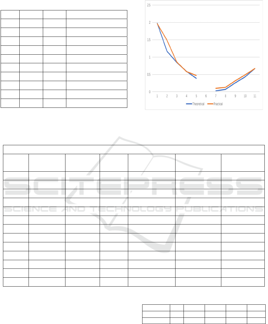
Table 7: Theoretical value (sigma is 0.424).
N(d1) N(d2) Theoretical value
Call 0.91 0.89 1.97
0.74 0.71 1.17
0.63 0.58 0.85
0.50 0.46 0.59
0.38 0.34 0.39
Put 0.62 0.66 0.03
0.09 0.11 0.07
0.26 0.29 0.26
0.37 0.42 0.43
0.50 0.54 0.67
As shown in the table above, the theoretical price
of option can be calculated from June.2,2022 to
June.22,2022 through Black-Scholes model.
Figure 1: Comparison between theoretical and practical
value.
Table 8: Error sum of squares of Black-Scholes model.
Black-Scholes model
6.1 sigma=0.424 Call K theoretical value practical value (P-Pm)^2/Pm
12 1.97 1.96 5.10204E-05
13 1.17 1.49 0.068724832
13.5 0.85 0.86 0.000116279
14 0.59 0.58 0.000172414
14.5 0.39 0.47 0.013617021
SSE 0.082681567
Put 11.5 0.03 0.1 0.049
12 0.07 0.13 0.027692308
13 0.26 0.32 0.01125
13.5 0.43 0.49 0.007346939
14 0.67 0.67 0
SSE 0.095289246
Total SSE 0.177970813
As shown in the figure above, for both call and put
options, the actual Ford Motor option prices are
generally higher than the theoretical values estimated
by the Black-Scholes model.
As shown in the table above, the sum of squares of
call option is 0.083 and put option is 0.095, the total
sum of squares of Black-Scholes model is 0.178. The
fitting result is valid. Based on the logical structure
and formulation of the model, the parameters of
Heston model can be calculated.
Table 9: Parameters of Heston model.
ρσ θ
k
v0
rho si
g
ma theta ka
pp
a v0
value 0 0.4326 0.6454 0.7376 0.193
As the table above shows, the volatility risk is 0,
the fluctuation in volatility is 0.4326, the mean of the
long run level is 0.6454, the rate of adjustment is
0.7376, and the variance of open price is 0.193. Hence,
after adjusting parameters, the Heston model can be
established.
Performance of Delta-Hedging on Black-Scholes Model and Heston Model
377

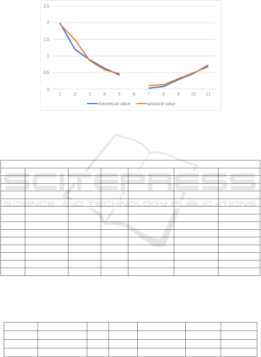
Figure 2: Comparisons between theoretical and practical value.
As shown in the figure above, this is a statistical
processing about the option price of Heston model.
For put option (in the right), most conditions practical
value is higher than theoretical value. While for call
option (in the left), both theoretical and practical value
have higher points.
Table 10: Error sum of squares of Heston model.
Heston model
6.1 sigma=0.433 Call K theoretical value practical value (P-Pm)^2/Pm
12 1.99 1.96 0.000459184
13 1.2 1.49 0.056442953
13.5 0.88 0.86 0.000465116
14 0.63 0.58 0.004310345
14.5 0.43 0.47 0.003404255
SSE 0.065081853
Put 11.5 0.03 0.1 0.049
12 0.08 0.13 0.019230769
13 0.29 0.32 0.0028125
13.5 0.47 0.49 0.000816327
14 0.72 0.67 0.003731343
SSE 0.075590939
Total SSE 0.140672792
As shown in the table above, the sum of squares of
call option is 0.065 and put option is 0.049, the total
sum of squares of Heston model is 0.141. The fitting
result is valid.
After establishing Black-Scholes model and
Heston model, do delta hedging based on the two
models and calculate the gain or loss from June.2,2022
to June.22,2022.
Table 11: Delta hedge of call option in Black-Scholes model.
date stock price(open) d1 N(d1) actual call price gain/loss total gain/loss
2022/6/2 13.64 2.05 0.98 1.48
0
-1.50
2022/6/3 13.63 2.12 0.98 1.32
-0.009796422
2022/6/6 13.74 2.64 1.00 1.34
0.108126984
ICEMME 2022 - The International Conference on Economic Management and Model Engineering
378

2022/6/7 13.26 1.88 0.97 0.97
-0.477996657
2022/6/8 13.63 2.74 1.00 1.19
0.358942818
2022/6/9 13.51 2.66 1.00 1.17
-0.119632467
2022/6/10 13 1.63 0.95 0.89
-0.508023709
2022/6/13 12.3 -0.31 0.38 0.41
-0.6637545
2022/6/14 11.99 -1.61 0.05 0.28
-0.117774181
2022/6/15 12.22 -0.86 0.20 0.34
0.012339877
2022/6/16 11.8 -3.29 0.00 0.17
-0.082143867
2022/6/17 11.24 -7.74 0.00 0.08
-0.000279742
2022/6/21 11.55 -29.82 0.00 0.03
0
2022/6/22
As the table above shows, the total loss of call
option in Black-Scholes model is 1.5, basically most
days in the red. On June.13,2022, it losses the most
which reaches 0.66 and on June,8,2022, it gains the
most which reaches 0.36.
Table 12: Delta hedge of put option in Black-Scholes model.
date stock price (open) d1 N(d1) actual put price gain/loss total gain/loss
2022/6/2 13.64 2.05 -0.02 0.19 0 0.59
2022/6/3 13.63 2.12 -0.02 0.24 0.000203578
2022/6/6 13.74 2.64 0.00 0.23 -0.001873016
2022/6/7 13.26 1.88 -0.03 0.25 0.002003343
2022/6/8 13.63 2.74 0.00 0.13 -0.011057182
2022/6/9 13.51 2.66 0.00 0.16 0.000367533
2022/6/10 13 1.63 -0.05 0.26 0.001976291
2022/6/13 12.3 -0.31 -0.62 0.57 0.0362455
2022/6/14 11.99 -1.61 -0.95 0.71 0.192225819
2022/6/15 12.22 -0.86 -0.80 0.5 -0.217660123
2022/6/16 11.8 -3.29 -1.00 0.9 0.337856133
2022/6/17 11.24 -7.74 -1.00 1.33 0.559720258
2022/6/21 11.55 -29.82 -1.00 0.9 -0.31
2022/6/22 1.09
As the table above shows, the total gain of put
option in Black-Scholes model is 0.59, basically most
days are profitable. On June.21,2022, it losses the
most which reaches 0.31 and on June,17,2022, it gains
the most which reaches 0.56.
Table 13: Delta hedge of put option in Heston model.
date stock price(open) delta actual put price gain/loss total gain/loss
2022/6/2 13.64 -0.20451 0.19 0 0.71153653
2022/6/3 13.63 -0.200254 0.24 0.0020451
2022/6/6 13.74 -0.1742165 0.23 -0.02202794
2022/6/7 13.26 -0.264333 0.25 0.08362392
2022/6/8 13.63 -0.178801 0.13 -0.09780321
2022/6/9 13.51 -0.194189 0.16 0.02145612
Performance of Delta-Hedging on Black-Scholes Model and Heston Model
379

2022/6/10 13 -0.3144005 0.26 0.09903639
2022/6/13 12.3 -0.5489845 0.57 0.22008035
2022/6/14 11.99 -0.670097 0.71 0.170185195
2022/6/15 12.22 -0.592458 0.5 -0.15412231
2022/6/16 11.8 -0.767487 0.9 0.24883236
2022/6/17 11.24 -0.9340715 1.33 0.42979272
2022/6/21 11.55 -0.91652 0.9 -0.289562165
2022/6/22 -0.94613 1.09
As the table above shows, the total gain of put
option in Heston model is 0.71, basically most days
are profitable. On June.21,2022, it losses the most
which reaches 0.29 and on June,17,2022, it gains the
most which reaches 0.43.
3.2 Discussion
As calculated and discussed above in the section about
result, the total sum of squares of Black-Scholes
model is 0.178 and the total sum of squares of Heston
model is 0.141. And the total gain of put option in
Heston model is 0.71 and the total gain of put option
in Black-Scholes model is 0.59. Therefore, the quasi
value of Heston's model is relatively more accurate
and profitable. The reason is that The Black-Scholes
model is an idealized model that does not perform so
well in practice since it has some flaws in its
assumptions. To illustrate, the model assumes that
stock prices follow a continuous geometric Brownian
motion, whereas in reality stock prices may jump like
the stock data from June.14.2022 to June.16,2022.
Moreover, if the stock price volatility specified by the
Black-Scholes model is constant, then the implied
volatility surface should be smooth which is
impossible. Nevertheless, relatively speaking, the
Heston model ensures the randomness of volatility. As
a result, the Heston model performs better than the
Black-Scholes model for the stock data of Ford Motor.
4 CONCLUSION
This paper mainly studies the effect of the same delta
hedging on Black-Scholes model and Heston model
using the same data about stock and option price of
Ford Motor. Although there are some researchers have
studied the difference and the pros and cons of the two
models, the topic which discuss the option price model
about Ford Motor has not been studied before. In this
paper, Black-Scholes model and Heston model are
established and be compared in terms of error sum of
squares and the total gain or loss. Firstly, an assumed
value of sigma is set and based on the logical structure
and formulation of the model, the theoretical value of
sigma is calculated. Then according to the model
established, the theoretical price of options are
calculated, Finally, using delta hedging, the total gain
or loss of the two models can be worked out and be
compared to analyses which model is more profitable
and suitable for Ford Motor.
However, since the status of dividends is not taken
into account, and the Black-Scholes model ignores the
transaction costs in real market, The results can be
significantly biased. In addition, apart from these two
models, there are many other famous option pricing
models like Cox-Ross-Rubinstein model, which
deserve more investigation in the future.
REFERENCES
D.K. Backus, S. Foresi, L. Wu. Accounting for biases in
Black-Scholes, 2004. Available at SSRN 585623.
J.D. MacBeth, L.J. Merville. An empirical examination of
the Black-Scholes call option pricing model. The
journal of finance, 1979, 34(5), 1173-1186.
J. Wu. Application of option pricing Theory in investment
decision of real estate development, 2004.
M. Bohner, Y. Zheng. On analytical solutions of the Black–
Scholes equation. Applied Mathematics Letters, 2009,
22(3), 309-313.
S.Y. Wang. Pricing European options in risk averse
markets, 2022.
W. S. Xie. Research on time fractional Asian option pricing
problem based on high precision finite difference
method, 2022.
Y.M. Liu. Application of option pricing theory in venture
capital, 2022.
Y.M. Liu. Application of option pricing theory in venture
capital, 2022.
Y. Qing. Numerical simulation and empirical analysis of
European option pricing model based on radial
function, 2022.
Z. Q. Lei, Q Zhong. Research on option pricing based on
uncertain fractional differential equation under floating
rate, 2022.
ICEMME 2022 - The International Conference on Economic Management and Model Engineering
380