
Algorithm and Model of Intelligent Classification for Optimizing the
Parameters of Beneficiation Technology
Andrey Kupin
1 a
, Dmytro Zubov
2 b
, Yuriy Osadchuk
1 c
and Vadym Saiapin
1 d
1
Kryvyi Rih National University, 11 Vitalii Matusevych Str., Kryvyi Rih, 50027, Ukraine
2
University of Central Asia, 310 Lenin Str., Naryn, 722918, Kyrgyzstan
Keywords:
Optimization, Beneficiation Processes, Magnetite Quartzite, Intellectual Classification and Control.
Abstract:
Based on the application of the classification control approach, a generalized algorithm for optimization of
beneficiation processes is proposed. The results of computer modelling of the classification optimization
process on the example of real indicators of magnetite quartzite beneficiation are presented. The results of
classification and evolutionary optimization procedures are compared. It was concluded that the proposed
intelligent classification method is able to determine the vector of settings and predict the TP beneficiation
with satisfactory accuracy. It is confirmed that the developed algorithms and control principles can be applied
to determine the required parameter values in modern ICS.
1 INTRODUCTION
The question of optimization of parameters of
technological process (TP) of magnetite quartzites
(iron ore) beneficiation in industrial conditions of the
mining and processing plant (MPP) for the purpose
of definition of settings of regulators as a part of
intelligent control system (ICS) is considered. The
multidimensional and multiconnected mathematical
model of TP, which is obtained as a result of the
identification procedure using the neural network
approach (Kupin and Senko, 2015), is considered to
be known. The relevance and general formulation of
such a task is presented in the works of the authors
(Bublikov and Tkachov, 2019; Kupin, 2014).
Various modifications of gradient algorithms are
now mainly used as search methods for multifactor
optimization of technological functions of targets,
optimal and adaptive automatic control systems
(AACS) (Morkun et al., 2018; Livshin, 2019).
However, it is well known that in the case of
poor conditionality of the optimization problem,
which is typical in the case of an attempt to
approximate technological functions (especially in
non-stationary processes), there are some problems
a
https://orcid.org/0000-0001-7569-1721
b
https://orcid.org/0000-0002-5601-7827
c
https://orcid.org/0000-0001-6110-9534
d
https://orcid.org/0000-0002-7415-5158
with the coincidence of the extremum search process
appear (Livshin, 2019). A good enough alternative to
this is the use of intelligent approaches: classification
control and evolutionary calculations (Rudenko and
Bezsonov, 2018; Trunov and Malcheniuk, 2018).
2 PROBLEM STATEMENT
Taking into account listed above, in the work
(Kupin, 2014) a combined ICS with multi-stage TP
beneficiation was developed. Features of the offered
decisions are a rational combination of approaches of
classification control and genetic optimization. The
purpose of this article is to develop a generalized
algorithm of intellectual classification, its research
by computer modelling and verification on the
principle of comparison with the results of genetic
optimization.
To implement the classification algorithm in terms
of TP beneficiation, we apply the problem statement
according to (Rudenko and Bezsonov, 2018). Let the
following categories be known in advance:
1) an alphabet of recognition classes for
technological situations in the form of a set
X
0
m
|m = 1,M
, (1)
which characterizes M functional states of TP and
let the class X
0
l
characterize the most desirable
Kupin, A., Zubov, D., Osadchuk, Y. and Saiapin, V.
Algorithm and Model of Intelligent Classification for Optimizing the Parameters of Beneficiation Technology.
DOI: 10.5220/0012008800003561
In Proceedings of the 5th Workshop for Young Scientists in Computer Science and Software Engineering (CSSE@SW 2022), pages 5-12
ISBN: 978-989-758-653-8; ISSN: 2975-9471
Copyright
c
2023 by SCITEPRESS – Science and Technology Publications, Lda. Under CC license (CC BY-NC-ND 4.0)
5

(search, close to ideal or quasi-optimal) state of
TP;
2) a training matrix of the type “object-property”,
which characterizes the m-th state of ICS in the
form
y
( j)
m,i
=
y
(1)
m,1
y
(1)
m,2
... y
(1)
m,l
... y
(1)
m,N
y
(2)
m,1
y
(2)
m,2
... y
(2)
m,l
... y
(2)
m,N
... ... ... ... ... ...
y
( j)
m,1
y
( j)
m,2
... y
( j)
m,l
... y
( j)
m,N
... ... ... ... ... ...
y
(n)
m,1
y
(n)
m,2
... y
(n)
m,l
... y
(n)
m,N
(2)
i = 1, N, j = 1,n, where each row is an
implementation of the image
n
y
( j)
m,i
|i = 1, N
o
and
the column of the matrix is a training sample from
the technological database (DB)
n
y
( j)
m,i
| j = 1, n
o
;
N, n are the numbers of signs of recognition and
testing (sample size), respectively.
In the result of training it is necessary to build a
division of the feature space into recognition classes
Ω in order to optimize and stabilize the functional
state of the ICS. In our case, for TP beneficiation
according to (Kupin and Senko, 2015), the feature
space is formed on the basis of the state vector of the
system, which contains all the necessary previously
normalized indicators (regime, control effects, output,
etc.).
3 RESULTS
Based on the above statement of the problem, the next
procedure of intellectual classification will have the
following stages.
1. The algorithm of intelligent classification
begins to work in case of a special situation (state).
This state is fixed when the current values of the initial
indicators (qualitative or quantitative i-th stage) at the
current (k-th) step of the system y
i
(k) are significantly
different from the planned settings y
∗
i
(k). That is,
none of the following conditions are met (or several
at a time):
| y
i
(k) − y
∗
i
(k) |≤ ∆
y
⇔
| Q
i
− Q
∗
|≤ ∆
Q
| β
i
− β
∗
|≤ ∆
β
| βx
i
− βx
∗
i
|≤ ∆
βx
, (3)
where Q
i
,β
i
,βx
i
are the current values of stage
productivity, the quality of the intermediate or
final product and the loss of useful in the tails,
respectively. In addition, the yield indicators (γ
i
) can
be additionally taken into account as similar criteria
and separation indicators (ε
i
). Q
∗
i
,β
∗
i
,βx
∗
i
are the
corresponding setting values. ∆Q,∆β, ∆βx are the
maximum permissible values of deviations between
the values of the settings and the corresponding output
values.
2. The main cause of special situations is
perturbations caused by constant fluctuations in the
quality composition and properties of primary raw
materials (charges) (Bublikov and Tkachov, 2019).
The peculiarity is that these effects in the conditions
of modern MPP are almost impossible to measure
accurately enough during the TP in real time.
Therefore, we apply the method of inverse prediction
using inverse models of short-term neural network
predictors (Kupin and Senko, 2015). For this purpose,
on the basis of the known values of the initial
indicators y
i
(k) from (3), obtained at the k-th step
of the system of the i-th stages, the corresponding
values of the input perturbations at the previous step
(k − 1) are predicted. Thus, the inverse model for the
neuroemulator has the form
v
i
(k − 1) ≈ ˆv
i
(k − 1) =
NN
−1
y
i
(k), y
i
(k − 1),...,y
i
(k − l
1
),
u
i
(k), u
i
(k − 1), ...,u
i
(k − l
2
− 1),
v
i
(k), v
i
(k − 1),...,v
i
(k − l
2
− 1)
,
(4)
where NN(·) is nonlinear function that performs
neural network transformation (direct or inverse,
depending on the direction of study); l
1
,l
2
are the
numbers of delayed signals at the input and output,
respectively.
The rest of the indicators, which are mode or
controlled, are determined by direct measurement by
appropriate means.
3. To implement the classification procedure, it
is necessary to form a sample of data for training
(parameterization) of the classifier. Such a sample is
formed on the basis of records of the technological
database, which is constantly updated during the
TP. Therefore, to improve the speed and quality
of training classifier with technological database
dimension M
DB
records is selected a limited cluster
with the number of C
S
records. In the process of
ISC, a neural network classifier is used, so the sample
size for training can be determined using expressions
from (Bublikov and Tkachov, 2019). Therefore, with
this in mind, the size of the cluster for classification
under TP beneficiation will be [180 ≤ C
S
≤ 900]. If
this amount of information is not in the technological
database (for example, at the beginning of the ICS),
the classification is impossible.
The selection of the specified number of cluster
elements from the technological database is by the
CSSE@SW 2022 - 5th Workshop for Young Scientists in Computer Science Software Engineering
6

method of the nearest neighbours based on the
analysis of vectors with a minimum value of the
Hamming radius (Rudenko and Bezsonov, 2018)
min
m
"
d
m
=
N
∑
i=1
(x
m,i
⊕ λ
i
)
#
, (5)
where x
m,i
is the i-th coordinate of the reference
(current) state vector from (1); λ
i
is the i-th coordinate
of an arbitrary vector from the technological database
that is a candidate for the cluster.
Therefore, as a result of a successful clustering
procedure, the C
S
of records (vectors) that are
closest (similar) to the current technological situation
according to criterion (5) will be selected for the
training sample (training cluster). In this case, as
alternative clustering methods the Kohonen network
or the principle of K-means may be used (Rudenko
and Bezsonov, 2018).
4. Synthesis and training of the classifying neural
network. Artificial neural networks today are one of
the most effective means for automatic classification
and clustering due to their sufficiently flexible
learning capabilities and generalization properties
(Kupin and Senko, 2015; Bublikov and Tkachov,
2019).
To solve the problem of classification (1) - (2), a
neural network based on a multilayer perceptron is
created (figure 1). The network contains 1-2 hidden
layers, the size of which is determined by setting up
the circuit empirically from a range of 18 ≤ n
h
≤ 450
neurons in total (Bublikov and Tkachov, 2019).
As a learning algorithm in the scheme (figure 1)
used one of the varieties of the algorithm with
inverse error propagation. An example of a two-class
classification shows that the root mean square error
(MSE) does not exceed 0.4 (Class 1) and 1.2 (Class
2). This indicates a sufficient quality of classification.
5. The main task in the course of classification
(or classification optimization) of the current
technological situation is the final choice from the
cluster of the best vector (X
∗
), which satisfies the
following two conditions:
• according to the input features most corresponds
to the current technological situation in the cluster
X
0
l
on the basis of the statement (1-2);
• according to the corresponding initial indicators
from the technological database best of all
corresponds to the value of the global criterion
type (7).
Therefore, on the basis of these conditions we
obtain
X
∗
= argexr
¯u(k), ¯v(k)
[J (y
1
(k + 1),y
2
(k + 1),y
3
(k + 1))
= J(Q,β,β
X
)],
(6)
where the criterion J(Q,β,β
X
) is selected by the
system or operator (technologist, dispatcher, etc.)
based on the modification of expression (7), for
example,
J(Q,β,β
X
) =
Q → max
β
min
≤ β ≤ β
max
β
min
X
≤ β
X
≤ β
max
X
, (7)
where Q is the output of the control stage or section;
β; β
min
; β
max
are the content of the useful component
and the corresponding restrictions (minimum and
maximum); β
X
; β
X
min
; β
X
max
are the loss of useful
in tails and corresponding restrictions.
The value of the expression of the main (first)
local criterion in expression (7) may change in the
process of ICS on a marginal principle. For example,
Q → max, β → max, β
X
→ min with restrictions on
the rest of the local criteria. Therefore, the ideal class
formed on the basis of (1-2) and (7) will have the form
X
0
l
:
y
( j)
m,l
=
n
Q
max
;β
max
;β
min
X
o
, (8)
where Q
max
the maximum value of the output
performance in the cluster.
With this in mind, the distribution function from
the current class analyzed in the classification process
will look like
S(X
0
m
) =
1(true),if
y
( j)
m,l
−y
( j)
m,i
y
( j)
m,l
< δ
K i
0(false),otherwise.
, (9)
where
δ
K i
|i = 1, N
is the limit values of control
tolerance fields for normalized recognition features.
After substitution (8) to (9) we obtain
S(X
0
m
) =
1,
h
Q
max
−Q
Q
max
< δ
Q
i
∧
h
β
max
−β
β
max
< δ
β
i
∧
h
β
min
X
−β
X
β
min
X
< δ
β
X
i
0
, (10)
where δ
Q
,δ
β
,δ
β
X
are the limit normalized values of
fields of control tolerances on the corresponding signs
of recognition (productivity, quality, losses); ∧ is
logical conjunction operation.
Functions (9 - 10) take only two logical values
of value: 1 (true - true), if the current class belongs
(close) to the ideal (8) or 0 (false) – otherwise
(technological situation is far from ideal).
6. Making a final decision on the suitability
(or unsuitability) of the classification results. For
the successful implementation of the automated
neural network classification procedure, the following
conditions must be consistently met:
Algorithm and Model of Intelligent Classification for Optimizing the Parameters of Beneficiation Technology
7
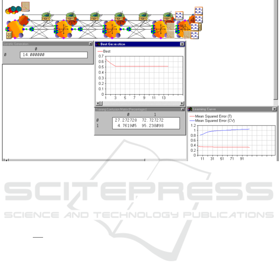
Figure 1: ICS classification neural network implemented in the environment of a specialized package of Neuro Solutions.
• the cluster for parameterization (training) of the
classifying neural network must contain not less
than the C
S
of vectors from the technological
database;
• if the precondition is fulfilled, it is necessary to
check the quality of classification on the basis of
calculating the value of the maximum measure of
control tolerance fields for normalized recognition
δ
K i
|i = 1, N
features defined (2) and allowable
forecast error ε
f
, which according to (Rudenko
and Bezsonov, 2018)
(
max [δ
K i
] ≤ δ
∗
K
ε
f
=
y(X
∗
) − y(X
0
l
)
≤ ε
∗
f
, (11)
where δ
∗
K
, ε
∗
f
are permissible values of tolerance
fields and forecast errors respectively.
• it is finally checked whether the obtained
classification solution X
∗
can satisfy the global
criterion of type (9), especially by constraints
(second and third local criteria).
If all these requirements are met, the final decision
on the success of the classification procedure is
made (return code 0 – “successful”). Otherwise, the
classification is impossible or unsuccessful (returns
an error code other than 0).
7. In case of successful classification according
to the algorithm, the class closest to the ideal
development of the technological situation according
to the global criterion is selected as a potential
solution (9).
Consider a computer model of the classification
algorithm for decision-making in the ISC on the
example of one stage of TP beneficiation. To do this,
we use a sample of statistical indicators of the second
stage in the 14-th section of the ore beneficiation plant
(OBP) No. 2 Southern MPP (Kryvyi Rih, Ukraine)
(Telenyk et al., 2018).
Table 1 shows an example of the current
technological situation (state vector X) at a certain
point in time. All factors are divided into three
groups:
1) a perturbations – input indicators that are not
subject to regulation at the current (second) stage
(output for the previous first stage);
2) the control effects and regime indicators that may
change or be regulated at the current stage;
3) the initial indicators to be optimized in the ICS at
the current stage in accordance with (9).
Therefore, in the first step, according to the
above algorithm, the cluster elements are selected
according to the degree of their similarity (proximity)
to the current technological situation (table 1) on the
basis of criterion (7). Table 2 shows a fragment of
such a cluster, which was selected from the current
technological database. The total volume of the
CSSE@SW 2022 - 5th Workshop for Young Scientists in Computer Science Software Engineering
8

Table 1: Instant sampling of indicators of the current technological situation.
№ Marking Explanation Value
1.1 d
1
,% Particle size distribution of the product at the output of the 1st stage by
class -0,074mm
48,57
1.2 Q
1
,t/h Processing (productivity) of the 1st stage of ore beneficiation 172,86
1.3 βnn
1
(β
1
),% Mass fraction (content) of total iron (magnetic) in the industrial product
of the 1st stage
47,64
1.4 βx
1
,% Loss of iron (mass fraction) in the tails of the 1st stage 12,98
1.5 γ
1
,% The yield of iron in the industrial product of the 1st stage 57,85
1.6 ε
1
,% Extraction (extraction) of iron in the industrial product of the 1st stage 85,28
2.1 C
2
,% Circulating load of the second stage 288,65
2.2 d
2
,% Particle size distribution of the intermediate product at the output of the
2nd stage of beneficiation by class -0,074mm
76,08
2.3 Ph
2
,% The solids content in the mill of the 2nd stage 76,85
2.4 ρ
k2
,% The density of the pulp in the TP classification of the 2nd stage
(hydrocyclone)
17,43
2.5 ρ
c2
,% The density of the pulp in the process of magnetic separation of the 2nd
stage
20,43
2.6 Bm
2
,t/h Water consumption in the mill of the 2nd stage 26,57
2.7 Bk
2
,t/h Water consumption in the hydrocyclone of the 2nd stage 102,86
2.8 Bc
2
,t/h Water consumption for magnetic separation of the 2nd stage 92,86
3.1 Q
2
,t/h Processing (productivity) of the 2nd stage of ore beneficiation 301,46
3.2 βnn
2
(β
2
),% Mass fraction (content) of total iron (magnetic) in the industrial product
of the 2nd stage
51,15
3.3 βx
2
,% Loss of iron (mass fraction) in the tails of the 2nd stage 10,17
3.4 γ
2
,% The yield of iron in the industrial product of the 2nd stage 65,74
3.5 ε
2
,% Extraction of iron in the industrial product of the 2nd stage 81,64
3.6 Q,t/h Productivity (average) for the processing of ore beneficiation 237,16
3.7 γ,% The yield of iron (average) for the processing of ore beneficiation 61,80
3.8 ε,% Extraction of iron (average) for the processing of ore beneficiation 83,46
Table 2: A fragment of a cluster with elements that best correspond to the current technological situation in the vector of input
indicators (perturbations).
№ d
1
,% Q
1
,t/h βnn
1
(β
1
),% βx
1
,% γ
1
,% ε
1
,% Criterion min[d
m
]
1 49,51 173,95 47,83 13,36 59,00 85,66 0,0802
2 48,98 178,73 47,59 12,88 57,56 85,18 0,0552
3 48,88 176,67 47,69 13,09 58,18 85,39 0,0433
4 48,82 179,67 47,55 12,80 57,31 85,10 0,0690
5 49,91 173,32 47,92 13,55 59,57 85,85 0,1123
6 49,62 175,61 47,76 13,23 58,61 85,53 0,0727
7 49,56 175,39 47,78 13,26 58,68 85,56 0,0744
8 48,94 171,89 47,93 13,57 59,61 85,87 0,0982
9 48,43 178,58 47,66 13,03 57,99 85,33 0,0416
10 48,55 171,03 47,98 13,66 59,90 85,96 0,1095
specified cluster, taking into account the requirements
(Bublikov and Tkachov, 2019) was C
S
= 250 records.
Therefore, the ideal class of initial (qualitative)
indicators, formed using the requirements (10) and
the data of table 3 will be as follows
y
( j)
m,l
=
n
Q
max
;β
max
;β
min
X
o
=
{
330;53, 3; 9,8
}
To automate the classification process, a
multilayer neural network of direct propagation
is used (figure 2), which is implemented in the
Neuro Solutions as neurosimulator. On the basis of
sample data from the cluster (tables 2-4) training
(parameterization) of the neural network is carried
out (figure 2).
To reduce the number of recognized classes in
the classification process, it is necessary to rationally
Algorithm and Model of Intelligent Classification for Optimizing the Parameters of Beneficiation Technology
9
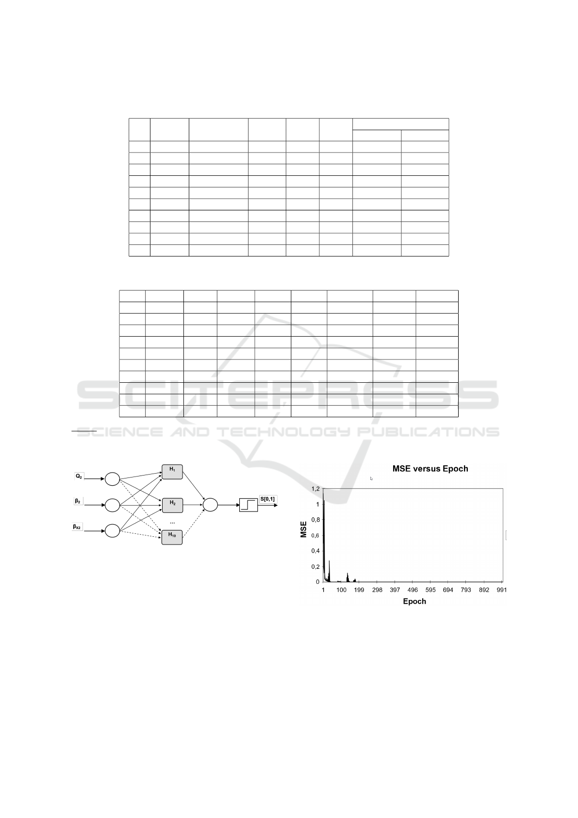
Table 3: A fragment of a cluster with elements that best correspond to the current technological situation in the vector of
output.
№ Q
2
,t/h βnn
2
(β
2
),% βx
2
,% γ
2
,% ε
2
,%
Limitation [min-max]
β
2
,% βx
2
,%
1 305,81 52,30 10,66 65,93 82,90 50,3-53,3 9,8-11,1
2 324,93 50,86 10,04 65,69 81,32 50,3-53,3 9,8-11,1
3 316,70 51,48 10,31 65,79 82,00 50,3-53,3 9,8-11,1
4* 328,69 50,61 9,93 65,65 81,04 50,3-53,3 9,8-11,1
5 303,31 52,87 10,91 66,02 83,53 50,3-53,3 9,8-11,1
6 312,47 51,91 10,50 65,86 82,48 50,3-53,3 9,8-11,1
7 311,58 51,98 10,53 65,88 82,55 50,3-53,3 9,8-11,1
8 297,56 52,91 10,93 66,03 83,58 50,3-53,3 9,8-11,1
9 324,34 51,29 10,23 65,76 81,79 50,3-53,3 9,8-11,1
10 294,15 53,20 11,05 66,08 83,89 50,3-53,3 9,8-11,1
Table 4: A fragment of a cluster with the corresponding elements according to the vector of control influences and mode
indicators.
№ C
2
,% d
2
,% Ph
2
,% ρ
k2
,% ρ
c2
,% Bm
2
,t/h Bk
2
,t/h Bc
2
,t/h
1 326,75 78,07 78,00 19,33 22,60 27,33 106,67 96,67
2 278,90 75,58 76,56 16,94 19,87 26,37 101,89 91,89
3 299,53 76,65 77,18 17,97 21,05 26,79 103,95 93,95
4** 270,38 75,13 76,31 16,51 19,39 26,20 101,03 91,03
5 345,86 79,06 78,57 20,29 23,69 27,71 108,58 98,58
6 313,97 77,40 77,61 18,69 21,87 27,07 105,39 95,39
7 316,19 77,52 77,68 18,80 22,00 27,12 105,61 95,61
8 347,32 79,14 78,61 20,36 23,77 27,74 108,73 98,73
9 293,27 76,33 76,99 17,66 20,69 26,66 103,32 93,32
10 356,73 79,63 78,90 20,83 24,31 27,93 109,67 99,67
Notes: where (*) is the class closest to the ideal on the basis of the analysis of values of initial (qualitative)
indicators; (**) is the corresponding vector of setting values (control effects and mode indicators) to ensure
quasi-optimal (close to ideal) output.
Figure 2: Neural network implementation scheme (3: 10:
1) for classification procedure.
choose the appropriate values of tolerance fields. This
can be done by varying the value of the tolerance and
its further study (figure 5).
As can be seen from figure 5 the number of classes
that are recognized linearly depends on the tolerance
values. This is evidenced by the linear trend, which is
determined on the basis of the known method of least
squares. The value of the coefficient of determination
R
2
= 99.8% indicates a sufficiently high reliability of
the approximation.
Analysis of the results of intellectual classification
Figure 3: Report on the course of parameterization of the
classification process.
(figures 3, 4, 5) and table 5 indicates the sufficient
quality of such a procedure. Thus, when changing the
normalized average tolerance fields within 4-4.5%, it
is possible to determine with sufficient adequacy from
1 to 13 vectors with potentially quasi-optimal settings
CSSE@SW 2022 - 5th Workshop for Young Scientists in Computer Science Software Engineering
10
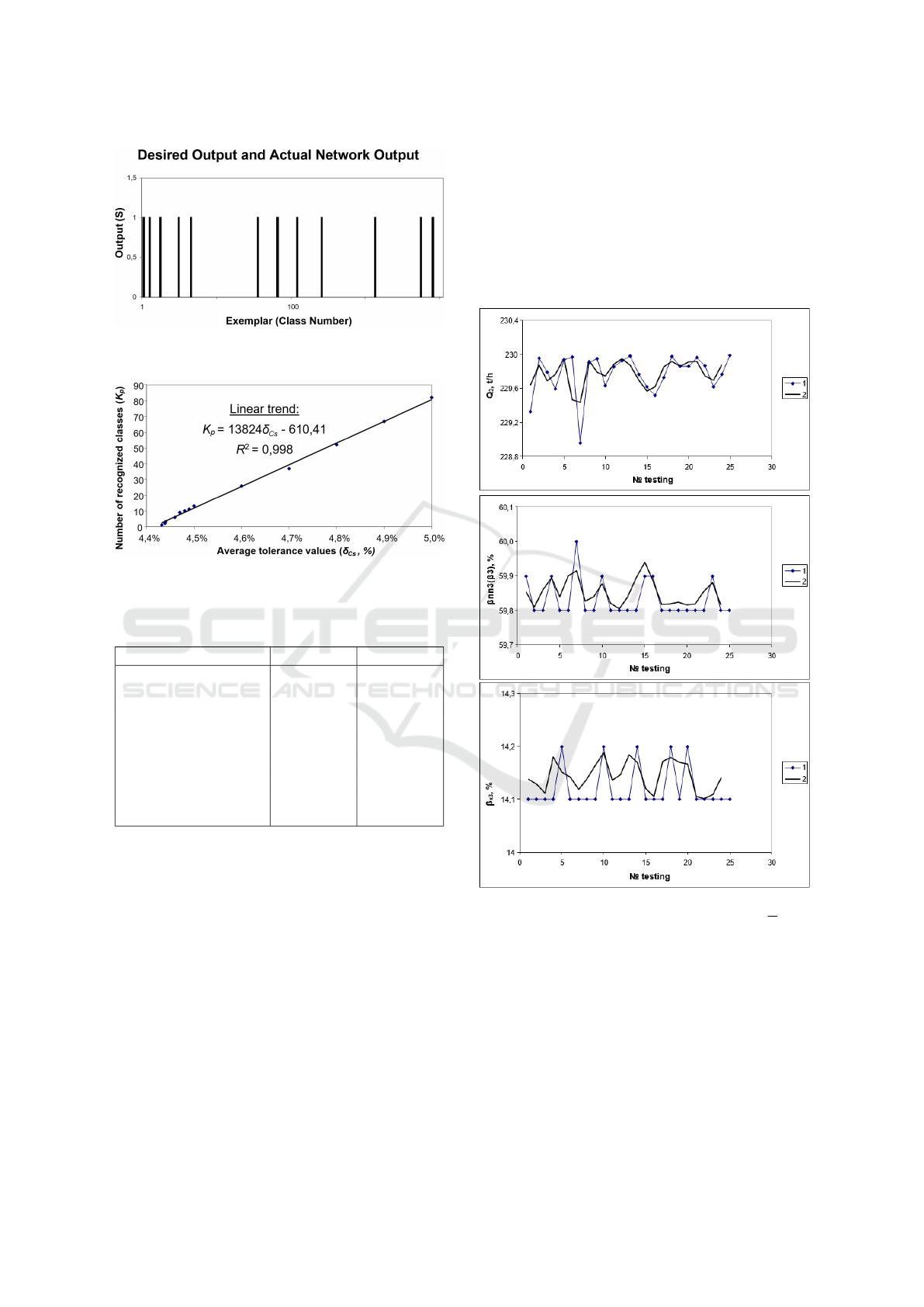
Figure 4: Report on the number of recognized classes in the
classification process.
Figure 5: Dependence of tolerance field values on the
number of recognized classes in the classification process.
Table 5: The resulting indicators of the adequacy of neural
network classification.
Marking (Input/ Output) S=0 S=1
1. MSE 1,49245E-10 3,78047E-07
2. NMSE 8,6783E-06 7,66892E-06
3. MAE 9,21927E-06 0,000205495
4. Min Abs Error 7,36317E-08 1,70942E-07
5. Max Abs Error 5,31987E-05 0,006554622
6. r 0,999995787 0,999996284
7. S=0 (rejected classes) 237 0
8. S=1 (classes are close
to ideal)
0 13
that are close to the ideal sample. In this case, based
on the application of the empirical linear dependence
of the trend, the quality of such a classification can
be significantly improved and brought to 1-3 samples.
The rate of convergence in the parameterization of the
circuit (figure 3) allows you to apply this approach in
real time.
Analysis of the results of the comparison of
dependencies (figure 6) shows their satisfactory
convergence. As expected, more accurate control
results are given by genetic optimization. On
the other hand, the classification approach has a
higher rate of coincidence. Therefore, both methods
have demonstrated the ability to determine the
required settings, both in the individual stages of TP
beneficiation, and for several stages simultaneously.
Depending on the quantity and quality of a priori
information in the technological database at the
current time it may be appropriate to use a certain
method. Therefore, the rational combination and
application in the ICS of two alternative strategies
(classification control and global optimization using
genetic algorithms) is appropriate and justified.
Figure 6: Comparative characteristics of the results of
classification and evolutionary optimization of the 3
rd
stage
of TP beneficiation of magnetite quartzites on productivity
(Q
3
) at restrictions on quality (β
3
) and losses in tails
(βx
3
): 1 – classification solution (Neuro Solutions); 2 –
optimization solution (NeuroShell2 + GeneHunter).
4 CONCLUSIONS
The analysis of results of computer modelling allows
to make certain generalisations in the form of such
Algorithm and Model of Intelligent Classification for Optimizing the Parameters of Beneficiation Technology
11

conclusions.
1. Intelligent classification using multilayer neural
networks and preceding cluster selection of the
training sample while ensuring the appropriate
number of cluster elements allows to determine
the vector of settings and predict the TP
beneficiation with satisfactory accuracy, which
relative error does not exceed the average
normalized tolerance field within 4-4.5%.
2. The results of computer simulation using
neurosimulators such as Neuro Solutions,
NeuroShell2 and genetic optimizer type
GeneHunter proved that the developed algorithms
and control principles using evolutionary
optimization methods, genetic algorithms and
automated intelligent classification can be applied
to the practical implementation of modern ICS in
conditions of complex multistage TP to determine
the required values of the settings.
REFERENCES
Aggarwal, C. C. (2018). Neural Networks and Deep
Learning. Springer Cham, London. https://doi.org/
10.1007/978-3-319-94463-0.
Bublikov, A. V. and Tkachov, V. V. (2019). Automation
of the control process of the mining machines based
on fuzzy logic. Naukovyi Visnyk Natsionalnoho
Hirnychoho Universytetu, 2019(3):112–118. https:
//doi.org/10.29202/nvngu/2019-3/19.
Hu, Z., Bodyanskiy, Y., and Tyshchenko, O. K. (2019).
Self-learning Procedures for a Kernel Fuzzy
Clustering System. In Hu, Z., Petoukhov, S.,
Dychka, I., and He, M., editors, Advances in
Computer Science for Engineering and Education,
pages 487–497, Cham. Springer International
Publishing. https://link.springer.com/chapter/10.
1007/978-3-319-91008-6 49.
Kupin, A. (2014). Research of properties of conditionality
of task to optimization of processes of concentrating
technology is on the basis of application of neural
networks. Metallurgical and Mining Industry,
6(4):51–55. https://www.metaljournal.com.ua/assets/
Journal/11.2014.pdf.
Kupin, A. and Senko, A. (2015). Principles of intellectual
control and classification optimization in conditions of
technological processes of beneficiation complexes.
CEUR Workshop Proceedings, 1356:153–160. https:
//ceur-ws.org/Vol-1356/paper 34.pdf.
Livshin, I. (2019). Artificial Neural Networks with Java.
Apress Berkeley, CA, 1 edition. https://doi.org/10.
1007/978-1-4842-4421-0.
Morkun, V., Morkun, N., Tron, V., and Dotsenko, I.
(2018). Adaptive control system for the magnetic
separation process. Sustainable Development
of Mountain Territories, 10(4):545–557. http:
//naukagor.ru/Portals/4/%233%202018/%E2%84%
964,%202018.pdf?ver=2019-02-21-091240-697.
Rudenko, O. G. and Bezsonov, A. A. (2018). Neural
network approximation of nonlinear noisy functions
based on coevolutionary cooperative-competitive
approach. Journal of Automation and Information
Sciences, 50(5):11–21. https://doi.org/10.1615/
JAutomatInfScien.v50.i5.20.
Semerikov, S. O., Vakaliuk, T. A., Mintii, I. S.,
Hamaniuk, V. A., Soloviev, V. N., Bondarenko, O. V.,
Nechypurenko, P. P., Shokaliuk, S. V., Moiseienko,
N. V., and Ruban, V. R. (2021). Development of the
computer vision system based on machine learning
for educational purposes. Educational Dimension,
5:8–60. https://doi.org/10.31812/educdim.4717.
Telenyk, S., Zharikov, E., and Rolik, O. (2018).
Modeling of the Data Center Resource Management
Using Reinforcement Learning. In 2018
International Scientific-Practical Conference
Problems of Infocommunications. Science and
Technology (PIC S&T), pages 289–296. https:
//doi.org/10.1109/INFOCOMMST.2018.8632064.
Trunov, A. and Malcheniuk, A. (2018). Recurrent network
as a tool for calibration in automated systems and
interactive simulators. Eastern-European Journal of
Enterprise Technologies, 2(9 (92)):54–60. https://doi.
org/10.15587/1729-4061.2018.126498.
CSSE@SW 2022 - 5th Workshop for Young Scientists in Computer Science Software Engineering
12
