Feature Selection of Hyperspectral Data Using an Improved Slime
Mould Algorithm
Hangjian Zhou
1
, Liancun Xiu
2
, Yule Hu
3
, Yingxu Xiao
4
and Zhizhong Zheng
5,*
1
School of Automation, China University of Geosciences, Wuhan, China
2
Nanjing Center, China Geological Survey, Nanjing, China
3
Faculty of Engineering, China University of Geosciences, Wuhan, China
4
School of Geophysics and Geomatics, China University of Geosciences, Wuhan, China
5
School of Computer Science, Nanjing University of Posts and Telecommunications, Nanjing, China
Keywords: Machine Learning, SMA, HYperspectral, Feature Selection.
Abstract: Hyperspectral data contains rich information but also has the problem of data redundancy, so it is necessary
to extract features from the data according to the application requirements to obtain useful waveform
information. Traditional hyperspectral data feature selection approaches rely on band screening and other
methods, which are imprecise and inefficient. Feature selection of hyperspectral data can be viewed as an
optimization process, and the Slime mould algorithm (SMA) in machine learning is an effective optimization
algorithm that simulates the foraging behavior of mucilaginous bacteria. In this paper, SMA is applied to the
feature selection of hyperspectral data, correlation information between the bands and the results is added to
the initial sampling process of the SMA, which speeds up the convergence of SMA and reduces the error of
feature selection. Based on the feature bands selected by this improved SMA, a hyperspectral soil heavy metal
inversion model was constructed, and the model was evaluated using three distinct evaluation methods: root
mean square error (RMSE), mean absolute error (MAE), and coefficient of determination (R2). The
experimental results demonstrate that the optimized model has faster convergence and less result error during
the feature selection phase, and that the final inversion model is more accurate.
1 INTRODUCTION
Hyperspectral data is the reflectance data of a sample
at multiple wavelengths obtained by measuring the
sample using a hyperspectral device, which has
hundreds of continuous bands. Since there are
differences in the reflectivity of matter for different
wavelengths of light, the subtle differences between
substances can be expressed through these hundreds
of bands (Bioucas-Dias et al., 2013). At the same
time, as a type of high-dimensional data,
hyperspectral data has the issue of redundant data, it
is required to extract features for the useful band
information within in (Xu et al., 2021).
Feature selection entails selecting the most
relevant variables from the data and eliminating other
variables that are weakly associated, hence enhancing
the accuracy of the model. In general, the feature
selection of the data is generally through two ways,
The first is the direct selection method, such as Liu et
al. direct selection of the feature band by the nature of
the substance (Liu et al., 2019), but its band selection
scheme is predefined, so its application scope is
limited. The other is the application of machine
learning algorithms for band selection, such as Lasso
regression algorithm (Li et al., 2018), Distance
Correlation (Li et al., 2012), Recursive Feature
Elimination (Gregorutti et al., 2017), etc. M.,Imani et
al. proposed a Fast Feature Selection Methods can
achieve the image classification accuracy (M. & H.,
2014), but there are still issues with the inversion of
the material. Zhang et al. applied the Ant Colony
Optimization to the feature selection process for soil
inversion of remote sensing pictures without taking
convergence speed into account (Zhang et al., 2019).
From an alternative viewpoint, the feature
selection problem can be viewed as an optimization
problem, i.e., selecting the few variables that have the
highest correlation with the results from multiple
variables; consequently, the band extraction process
of Hyperspectral can be viewed as an optimization
process. Li et al. proposed the
Slime Mould Algorithm
644
Zhou, H., Xiu, L., Hu, Y., Xiao, Y. and Zheng, Z.
Feature Selection of Hyperspectral Data Using an Improved Slime Mould Algorithm.
DOI: 10.5220/0012007000003612
In Proceedings of the 3rd International Symposium on Automation, Information and Computing (ISAIC 2022), pages 644-650
ISBN: 978-989-758-622-4; ISSN: 2975-9463
Copyright
c
 2023 by SCITEPRESS – Science and Technology Publications, Lda. Under CC license (CC BY-NC-ND 4.0)

(SMA) in 2020 as an new population intelligence
optimization algorithm (Li et al., 2020). By varying
the weight, they simulated the positive and negative
feedback processes in the slime mold foraging
process. The approach has been frequently applied to
optimization problems because of its convergence
precision and stability. For instance, Wei et al.
successfully applied it to The Optimal Reactive
Power Dispatch (ORPD) proble (Wei et al., 2021).
In response to the above problems, the improved
SMA is applied to the feature selection of
hyperspectral data, and a hyperspectral soil heavy
metal inversion model is developed based on the
feature bands extracted by the optimized algorithm in
this paper.
The main contributions of this paper are as
follows.
1) By treating the feature selection problem as
an optimization problem, the SMA is applied
in feature selection of hyperspectral data to
obtain useful bands information.
2) further improvement of SMA is achieved by
adding the correlation information between
the bands and the results to the initial
sampling process of SMA by using the
Spearman's rank correlation coefficient.
3) On the basis of the Support Vector Machine
(SVM) regression algorithm, three
hyperspectral soil heavy metal inversion
models were built and evaluated using three
distinct evaluation methodologies.
The rest of the paper is organized as follows. In
the second section, the algorithm is optimized and an
inverse model is developed. A series of experiments
and analyses are given in the third section. Finally,
the fourth section summarizes the paper.
2 METHOD
2.1 Slime Mould Algorithm (SMA)
The SMA is a metaheuristic algorithm with great
merit-seeking abilities and rapid convergence (Li et
al., 2020). The operation of the SMA consists of three
main stages. The first is random diffusion to find the
food with the strongest odor, then approaching
diffusion toward the food with the strongest odor, and
finally completing the wrapping of the target. The
mathematical operation may imitate the random
motion with directionality displayed by slime bacteria
during their quest for food, and when this random
motion tends to be stable, the slime bacteria position
is the optimal value chosen by the slime bacteria
algorithm. This motion's iterative pattern can be
described by Eq. (1).
𝑋
(
𝑡+1
)
=

𝑟𝑎𝑛𝑑.
(
𝑈𝐵 − 𝐿𝐵
)
+𝐿𝐵,𝑟𝑎𝑛𝑑<𝑧
𝑋

+𝑣

∗

𝑊∗𝑋

(
𝑡
)
−𝑋

(
𝑡
)

,𝑟𝑎𝑛𝑑<𝑝
𝑣

∗𝑋
(
𝑡
)
,𝑟𝑎𝑛𝑑<𝑝
(1)
where the parameters of p are as follows：
𝑝=𝑡𝑎𝑛ℎ
|
𝑆(𝑖)−𝐷𝐹
|
(2)
Among Eq. (2), 𝑆(𝑖) is the fitness score of the 𝑖-
th particle in this iteration, and 𝐷𝐹 is the optimal
fitness score since the beginning of the iteration.𝑈𝐵
and 𝐿𝐵 are the upper and lower boundaries of the
optimization search space, while 𝑧 is a threshold
parameter with a relatively low value. 𝑋

is the
position of the slime bacteria with the highest
concentration of food odor found at the current
moment, i.e., the current optimal solution. 𝑣

is a
random value in the interval [-𝑎, 𝑎], and the value of
𝑎 is as follows.
𝑎=𝑎𝑟𝑐𝑡𝑎𝑛((−

_
)+1) (3)
As the iteration count grows, 𝑣

declines linearly
from 1 to a random value between 0 and 1.
The expression for 𝑊 in Eq. (1) is shown below:
𝑊=
1+𝑟∙𝑙𝑜𝑔


(

)

+1

,𝑐𝑜𝑛𝑑𝑖𝑡𝑜𝑛𝑠
1−𝑟∙𝑙𝑜𝑔


(

)

+1

,𝑜𝑡ℎ𝑒𝑟𝑠
(4)
Eq. (4) is contingent on 𝑆
(
𝑖
)
's size being in the
top half of all particles' rankings during the current
iteration. The best fitness score for this iteration is
𝑏𝐹, while the poorest fitness score is 𝑤𝐹.
During the preceding procedure, the particle
positions gradually converge to the optimal aim as the
number of iterations increases.
2.2 Application of SMA to Feature
Selection
The hyperspectral data can be considered as a series
of high-dimensional vectors 𝐴=

𝑎

,𝑎

…𝑎

…𝑎


， where 𝑎

is the spectral reflectance of the 𝑖-th
band. Feature selection on hyperspectral data consists
of selecting 𝑚 elements from 𝑛 elements to
construct a new vector set 𝐵=

𝑏

,𝑏

,…,𝑏


(
𝑚<
𝑛
)
. In the ensuing modeling phase, vector 𝐵 is
Feature Selection of Hyperspectral Data Using an Improved Slime Mould Algorithm
645

modeled in place of vector 𝐴, thereby eliminating
redundant data.
The application of the traditional SMA is still
limited to the selection of optimal values within a
certain range, whereas the feature selection problem
is to select the most pertinent variables from the data.
Therefore, the algorithm must be further optimized to
address the feature selection problem.
In terms of the nature of the problem, the selection
behavior of the data variables can be understood as a
process of binarization, i.e., being selected when the
value is 1 and not being picked when the value is 0.
Therefore, the optimization issue can be transformed
into a problem involving feature selection.
For the band selection model of hyperspectral
data, the dimensionality of the particles is first
determined to ensure that the number of dimensions I
of the particles equals the number of bands n of the
data. In addition, the upper limit 𝑈𝐵 and lower limit
𝐿𝐵 of search seeking must be set to 1 and 0
correspondingly, and a threshold 𝜆 must be set so
that each 𝑋

satisfies Eq. (5), thereby expressing the
relationship between the selection of particles and the
selected ones.
𝑋

=
0,𝜆<0.5
1,𝜆≥0.5
(5)
By configuring this relationship, the particle
values are binarized in order to select the desired
band. In addition, the fitness score within the SMA
must be specified. In the process of selecting features
for hyperspectral data, the level of the fitness score
corresponds to the merit of various band selection
schemes. Here, the partial least squares regression
(PLSR) model, which requires few setup parameters
and is efficient, is introduced for quantitative
evaluation of feature selection schemes. Specifically,
the data corresponding to the specified bands are
modeled with the data to be inverted using PLSR, and
the root mean square error (RMSE) score of the
resulting model is utilized as the fitness value. As a
result, the level of the fitness score can express the
advantages and disadvantages of different band
selection schemes.
𝑅𝑀𝑆𝐸=



∑
(𝑦

−𝑦

)


(6)
Where 𝑦

and 𝑦

 represent the true value and
predicted value of the 𝑖-th sample respectively. This
band selection strategy is more successful when
RMSE has a smaller value.
2.3 Sampling-Optimized Slime Mould
Algorithm (SO-SMA)
When band selection is performed for hyperspectral
data, the initial sampling process of SMA discussed
above is a uniform sampling with a threshold of 0.5.
However, for hyperspectral data, the value of each
band has a considerable effect on the findings,
therefore the threshold needs to be continuously
modified for different bands. In this research, the
Spearman’s rank coefficient of correlation is used to
express the effect of each band on the results. In the
initial sampling process of the SMA, the acceptance-
rejection sampling with correlation coefficient as the
threshold is used in place of the original uniformly
distributed sampling to improve the initial state of the
algorithm and increase the directionality in the feature
selection process. The algorithm after sampling
optimization strategy has the potential to expedite the
convergence of the algorithm for feature selection.
The Spearman's rank correlation coefficient
which is denoted by the Greek letter 𝜌 in this work
is used to estimate the correlation between two
variables 𝑋 and 𝑌, where the correlation between
the variables can be described using a monotonic
function (Schober et al., 2018). The correlation
coefficient between two variables can be either +1 or
-1 if one of their respective sets of values can be
adequately represented by the other variable as a
monotonic function (i.e., the two variables have the
same trend of change).
Suppose that the two random variables are 𝑋 and
𝑌 respectively, the number of their elements are both
𝑁. The 𝑖-th value taken by 𝑋 and 𝑌 is denoted by
𝑋

and 𝑌

respectively. 𝑥

and 𝑦

are the ordered
set of elements in 𝑋 and 𝑌. 𝑑

is a ranking
difference set after the corresponding subtraction of
the elements in the sets 𝑥

and 𝑦

. Finally, as shown
in Eq. (7), a simpler procedure is used to calculate 𝜌.
𝜌=1−

∑



(

)
(7)
𝑑

=𝑥

−𝑦

， 1≤𝑖≤𝑁 (8)
After computing the Spearman's rank correlation
coefficient independently for each band, it is
necessary to linearly deflate the absolute values of the
acquired correlation coefficients in order to give a
more effective sampling optimization. In this paper,
the maximum value of correlation coefficient after
linear reduction is 0.8 and the minimum value is 0.2.
Eventually, they become the selected thresholds for
ISAIC 2022 - International Symposium on Automation, Information and Computing
646

each band in the feature selection process. As shown
in the Eq. (9).
𝑋

=
𝑆𝑒𝑙𝑒𝑐𝑡𝑒𝑑, 𝜆<𝑡ℎ𝑟𝑒

𝑈𝑛𝑠𝑒𝑙𝑒𝑐𝑡𝑒𝑑, 𝜆≥𝑡ℎ𝑟𝑒

(9)
Eq. (9) permits the selection of the band with the
highest absolute correlation coefficient with an 80%
chance during the initial phase of the SMA. Similarly,
the band with the lowest correlation with the result
has a 20% chance of being chosen in the initial
procedure ， which brings the algorithm's random
distribution near to the distribution of the correlation
coefficient.
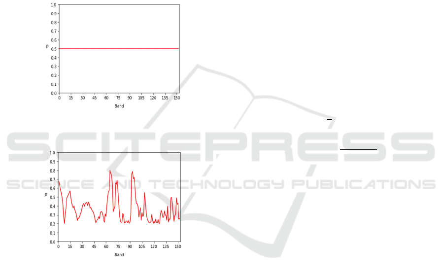
Figure 1: The probability of each band being selected
before algorithm optimization.
Figure 2: The probability of each band being selected after
algorithm optimization.
In Fig. 1 and Fig. 2, 𝑝 is the probability of the
band being selected. As shown in the picture, the
sampling-optimized SMA (SO-SMA) is more
relevant for different bands and the correlation
between the bands and the outcomes influences the
selection of different bands.
2.4 Inversion Method
In this study, the inversion model is built with the
SVM regression algorithm, a branch of the normal
SVM algorithm. The objective of the SVM regression
algorithm is to locate the ideal hyperplane that brings
the data closest to the hyperplane and enables
regression analysis via data fitting. The advantage of
the SVM regression algorithm is that only a small
number of support vectors are required to establish
the optimal hyperplane, and the kernel method
endows the data with a nonlinear regression
approach; therefore, it has a distinct advantage when
dealing with small samples of high-dimensional
hyperspectral data (Yuan et al., 2017). In the
subsequent experiments, this paper uses the SVM
regression algorithm to model the inversion of
hyperspectral soil heavy metals based on the data
extracted by the SMA and the SO-SMA in the
previous paper.
2.5 Model Evaluation Method
In this study, three evaluation metrics, root mean
square error (RMSE), mean absolute error (MAE), and
coefficient of determination (R2)
, are chosen to evaluate
the inversion model constructed using SMA
following the initial sampling optimization.
RMSE is
defined by Eq. (6), MAE and R2 are defined as
follow.
𝑀𝐴𝐸=


∑
𝑦

−𝑦




(10)
𝑅

=1−
∑
(




)


∑
(






)


(11)
Where 𝑦

and 𝑦

 represent the true value and
predicted value of the 𝑗-th sample respectively, 𝑦


is the average of the true value, and 𝑁 is the number
of samples. The three evaluation indices are identified
by the letters C and P in the bottom right-hand corner
of the model training and prediction data sets (from
the initials Calibration and Prediction, respectively).
That is, we've lettered the assessments of the training
data sets 𝑅


, 𝑅𝑀𝑆𝐸

and 𝑀𝐴𝐸

, and the
assessments of the prediction data sets 𝑅


, 𝑅𝑀𝑆𝐸

and 𝑀𝐴𝐸

.
3 EXPERIMENTAL EVALUATION
3.1 Study Area and Datasets
As shown in Fig. 3, the area chosen for this study is
situated on the northern bank of the Yangtze River in
the Chinese city of Nanjing, Jiangsu Province. The
presence of nearby heavy industrial facilities may
result in the enrichment of heavy metals in the
surrounding soil. In this paper, 134 ground soil
sampling sites in the study region were selected, and
Feature Selection of Hyperspectral Data Using an Improved Slime Mould Algorithm
647

modeling inversions were done based on the relevant
data of laboratory-measured heavy metal
concentrations and the hyperspectral data of the
sample sites' corresponding locations.
Figure 3: Study area and location of sampling points.
Three different types of soil heavy metals were
statistically examined. The results are displayed in
Table 1.
Table 1: Descriptive statistics of heavy metal concentration.
Cd
( mg/kg ) Cu ( mg/kg ) Hg ( 10
-3
mg/kg )
Max 50.995 148.1 175.65
Min 19.3 80.0 37.3
Mean 33.34 106.38 101.49
Std 6.29 11.58 21.60
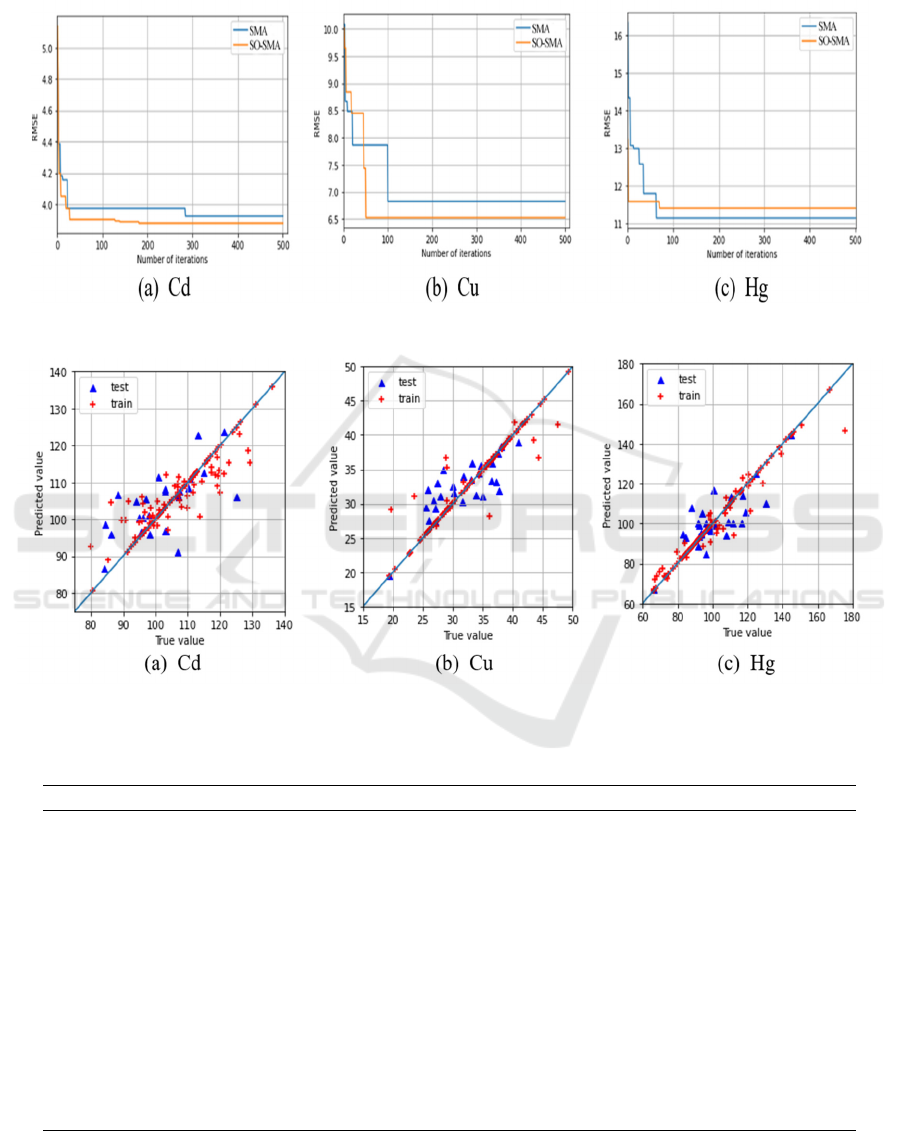
3.2 Rate of Convergence
In this paper, we use SMA and SO-SMA for feature
selection of hyperspectral data of three different
heavy metals. From the results of the feature selection
of part (a) and part (b) in Fig. 4, it can be inferred that
the SO-SMA is indeed consistent with fast
convergence in terms of feature selection of spectral
data, and the RMSE error is also reduced. For the
convergence results of part (c) in Figure 3, SMA and
SO-SMA only took a fewer number of iterations to
get a smaller RMSE due to the limited data of the
measured samples and the weak content of Hg in the
soil, which caused SO-SMA to lack a noticeable
advantage.
The intention of the Spearman's rank correlation
coefficient utilized in this research for the
construction process of acceptance-rejection
sampling is to circumvent the inadequacies of
Pearson correlation coefficients. This is due to the
fact that the Pearson correlation coefficient may not
fulfill the normal distribution in the case of a small
sample size, and therefore fails to meet the common
assumption of its correlation coefficient. The
Spearman's rank correlation merely demands that the
observations of the two variables be paired rank-rated
information or that the rank information be derived
from observations of continuous variables.
Consequently, regardless of the general distribution
pattern of the two variables and the sample size, the
Spearman rank correlation coefficient may be utilized
to assess the correlation between the two variables. In
the optimization process of the SMA, this paper
stretches the absolute value of the Spearman's rank
correlation coefficient and applies it to the initial
sampling process of the SMA, thereby transforming
the uniform distribution in the band selection process
into a dynamic distribution that varies according to
the relationship between the band and the result.
Therefore, the SO-SMA achieves superior outcomes
in the hyperspectral data feature selection procedure.
3.3 Model Evaluation
Based on the original data, the data after feature
selection by SMA, and the data after feature selection
by SO-SMA, and using the SVM regression
algorithm, hyperspectral soil heavy metal inversion
models (SVM, SMA-SVM and SO-SMA-SVM) were
built in this paper. In addition, Recursive Feature
Elimination (REF), a classic feature selection
approach in machine learning, is also frequently
utilized in band extraction of hyperspectral data;
therefore, this study establishes an RFE-SVM
inversion model based on this algorithm. Firstly, all
of the samples were separated into training sets and
test sets. The training set was used to tweak the
model's parameters and establish the model, while the
test set was used to assess the model's generalization
capacity. Tabulated in Table 2 are the precisions of
the 4 models. Finally, the inversion model was
evaluated using the RMSE, MAE, and R2 assessment
indices.
From the inversion model accuracy table, it is
clear that the SVM regression method suffers from
overfitting throughout the inversion model
development process and is therefore incapable of
completing the soil heavy metal inversion accurately
and effectively. In addition, the REF-SVM model
developed based on REF can only partially mitigate
the overfitting issue, and the accuracy is low, so the
effect of the inversion process is not adequate. In
contrast, the SMA-SVM and SO-SMA-SVM models
ISAIC 2022 - International Symposium on Automation, Information and Computing
648

built by using the SMA for feature selection of
hyperspectral data both weakened the overfitting
phenomenon. Comparing the SMA-SVM and SO-
SMA-SVM models, the SO-SMA-SVM model
generated after the initial sampling optimization
provides more accurate end findings than the SMA-
SVM model.
Figure 4: Comparison of optimal RMSE changes in every iteration.
Figure 5:
Inversion scatter diagram of SO-SMA-SVM model.
Table 2: Regression results of SVM, SMA-SVM and SO-SMA-SVM.
Metal Method
𝑅


𝑅𝑀𝑆𝐸

𝑀𝐴𝐸

𝑅


𝑅𝑀𝑆𝐸

𝑀𝐴𝐸

Cd SVM 0.99 0.09 0.09 0.48 3.60 2.96
REF-SVM 0.99 0.09 0.08 0.51 3.41 2.84
SMA-SVM 0.97 0.15 0.12 0.53 3.53 2.77
SO-SMA-SVM 0.89 2.03 1.69 0.61 3.02 2.06
Cu SVM 0.84 4.35 2.26 0.43 6.39 8.28
REF-SVM 0.83 4.28 2.15 0.47 6.37 7.75
SMA-SVM 0.83 4.21 2.35 0.59 6.33 6.98
SO-SMA-SVM 0.81 4.85 2.74 0.62 6.21 6.35
Hg SVM 1.00 0.10 0.10 0.49 11.49 9.31
REF-SVM 0.99 0.10 0.10 0.49 11.12 9.02
SMA-SVM 0.95 0.11 0.12 0.51 10.45 8.77
SO-SMA-SVM 0.94 0.14 0.16 0.63 9.34 7.21
Feature Selection of Hyperspectral Data Using an Improved Slime Mould Algorithm
649

4 CONCLUSIONS
This work employs the SMA method for feature
selection of hyperspectral data in order to overcome
the problem of data redundancy encountered during
the information extraction process of hyperspectral
data. This paper replaces the uniformly distributed
sampling in the initial randomization process of the
SMA with acceptance-rejection sampling during the
feature selection procedure, thereby incorporating the
relationship between the waveband and the result into
the algorithm during the optimization phase and
enhancing the algorithm's convergence speed and
precision. In addition, we applied the SO-SMA to the
hyperspectral soil heavy metal inversion modeling
procedure, and the final experimental results
demonstrated that the final results of the optimized
sampling feature selection algorithm were superior to
those of the most fundamental uniformly distributed
sampling feature selection scheme, and diminished
the overfitting phenomenon in the conventional SVM
model. Therefore, before selecting features for the
bands of hyperspectral data, it is essential to consider
the correlation coefficient of each band for the
outcomes.
ACKNOWLEDGEMENTS
This work was supported by Jiangsu Province Natural
Resources Development Special Fund (Marine
Science and Technology Innovation) Project (Grant
No. JSZRHYKJ202007) and Jiangsu Province
Frontier Leading Technology Basic Research Project
(Grant No. BK20192003).
REFERENCES
Bioucas-Dias, J. M., Plaza, A., Camps-Valls, G.,
Scheunders, P., Nasrabadi, N. M., & Chanussot, J.
(2013). Hyperspectral Remote Sensing Data Analysis
and Future Challenges. IEEE Geoscience and Remote
Sensing Magazine, 1(2), 6-36.
http://doi.org/10.1109/MGRS.2013.2244672
Gregorutti, B., Michel, B., & Saint-Pierre, P. (2017).
Correlation and variable importance in random forests.
STATISTICS AND COMPUTING, 27(3), 659-678.
http://doi.org/10.1007/s11222-016-9646-1
Li, J. D., Cheng, K. W., Wang, S. H., Morstatter, F.,
Trevino, R. P., Tang, J. L., & Liu, H. (2018). Feature
Selection: A Data Perspective. ACM COMPUTING
SURVEYS, 50(6) http://doi.org/10.1145/3136625
Li, R. Z., Zhong, W., & Zhu, L. P. (2012). Feature
Screening via Distance Correlation Learning.
JOURNAL OF THE AMERICAN STATISTICAL
ASSOCIATION, 107(499), 1129-1139.
http://doi.org/10.1080/01621459.2012.695654
Li, S. M., Chen, H. L., Wang, M. J., Heidari, A. A., &
Mirjalili, S. (2020). Slime mould algorithm: A new
method for stochastic optimization. Future Generation
Computer Systems-The International Journal of
eScience, 111, 300-323.
http://doi.org/10.1016/j.future.2020.03.055
Liu, Z., Lu, Y., Peng, Y., Zhao, L., Wang, G., & Hu, Y.
(2019). Estimation of Soil Heavy Metal Content Using
Hyperspectral Data Remote Sensing (11, pp.).
M., I., & H., G. (2014, 0009-11-20). Fast feature selection
methods for classification of hyperspectral images.
Paper presented at the 7'th International Symposium on
Telecommunications (IST'2014).
Schober, P., Boer, C., & Schwarte, L. A. (2018).
Correlation Coefficients: Appropriate Use and
Interpretation. ANESTHESIA AND ANALGESIA,
126(5), 1763-1768.
http://doi.org/10.1213/ANE.0000000000002864
Wei, Y. Y., Zhou, Y. Q., Luo, Q. F., & Deng, W. (2021).
Optimal reactive power dispatch using an improved
slime mould algorithm. Energy Reports, 7, 8742-8759.
http://doi.org/10.1016/j.egyr.2021.11.138
Xu, M. Z., Liang, S., Shi, J. L., Ji, Y., Huang, Y., Liang, S.
Y., & Yan, W. (2021). Airborne hyperspectral
inversion of heavy metal distribution in cultivated soil:
A case study of Guanhe area, northern Jiangsu Province.
East China Geology, 42(1), 100-107.
http://doi.org/10.16788/j.hddz.32-1865/P.2021.01.012
Yuan, H. H., Yang, G. J., Li, C. C., Wang, Y. J., Liu, J. G.,
Yu, H. Y., Feng, H. K., Xu, B., Zhao, X. Q., & Yang,
X. D. (2017). Retrieving Soybean Leaf Area Index from
Unmanned Aerial Vehicle Hyperspectral Remote
Sensing: Analysis of RF, ANN, and SVM Regression
Models. Remote Sensing, 9(4)
http://doi.org/10.3390/rs9040309
Zhang, Y., Li, M., Zheng, L., Qin, Q., & Lee, W. S. (2019).
Spectral features extraction for estimation of soil total
nitrogen content based on modified ant colony
optimization algorithm. GEODERMA, 333, 23-34.
http://doi.org/10.1016/j.geoderma.2018.07.004
ISAIC 2022 - International Symposium on Automation, Information and Computing
650