Sentiment Analysis of Electronic Social Media Based on Deep Learning

Vasily D. Derbentsev

1 a

, Vitalii S. Bezkorovainyi

1 b

, Andriy V. Matviychuk

1 c

Oksana M. Pomazun

1 d

, Andrii V. Hrabariev

1 e

and Alexey M. Hostryk

2 f

Kyiv National Economic University Named After Vadym Hetman, 54/1 Peremogy Ave., Kyiv, 03680, Ukraine

Odessa National Economic University,8 Preobrazhenskaya Str., Odessa, 65082, Ukraine

Keywords:

Sentiment Analysis, Social Media, Deep Learning, Convolutional Neural Networks, Long Short-Term

Memory, Word Embeddings.

Abstract:

This paper describes Deep Learning approach of sentiment analyses which is an active research subject in the

domain of Natural Language Processing. For this purpose we have developed three models based on Deep

Neural Networks (DNNs): Convolutional Neural Network (CNN), and two models that combine convolutional

and recurrent layers based on Long-Short-Term Memory (LSTM), such as CNN-LSTM and Bi-Directional

LSTM-CNN (BiLSTM-CNN). As vector representations of words were used GloVe and Word2vec word em-

beddings. To evaluate the performance of the models, were used IMDb Movie Reviews and Twitter Sentiment

140 datasets, and as a baseline classiﬁer was used Logistic Regression. The best result for IMDb dataset

was obtained using CNN model (accuracy 90.1%), and for Sentiment 140 the model based on BiLSTM-CNN

showed the highest accuracy (82.1%) correspondinly. The accuracy of the proposed models is a quite accept-

able for practical use and comparable to state of the art models.

1 INTRODUCTION

The rapid development of electronic mass media and

social networks has given a new impetus to the de-

velopment of automated Natural Language Process-

ing (NLP) systems.

NLP is an interdisciplinary ﬁeld at the intersection

of Computer Science, Artiﬁcial Intelligence and Lin-

guistics, dedicated to how computers analyze natural

(human) language models.

The range of tasks that NLP solves is quite wide.

For example, NLP can be used to build automatic

systems like machine translation, speech recognition,

named entity recognition, text classiﬁcation and sum-

marization, sentiment analysis, question answering,

autocomplete, predictive text input, and so on (N1,

2021; Mayur et al., 2022; N43, 2018).

One of the important tasks of NLP is Sentiment

Analysis (SA), also known as opinion mining. SA is

https://orcid.org/0000-0002-8988-2526

https://orcid.org/0000-0002-4998-8385

https://orcid.org/0000-0002-8911-5677

https://orcid.org/0000-0001-9697-1415

https://orcid.org/0000-0001-6165-0996

https://orcid.org/0000-0001-6143-6797

an attempt to extract subjective characteristics from

the text: emotions, sarcasm, confusion, suspicion etc.

The main goal of SA is to classify the polarity of a

given document, and to determine whether the opin-

ion expressed in a document or sentence is positive,

negative, or neutral.

It is a very popular text classiﬁcation technique

because sentiment can convey a wealth of informa-

tion about one’s point of view on a subject under dis-

cussion. It helps to conduct a comprehensive anal-

ysis of feedback, polarity of messages or reactions.

SA is widely used among businessmen, marketers and

politicians.

In the analysis of public opinion on sensitive so-

cial and political issues, identifying common themes

and tone of discussion can greatly simplify the work

of experts in the ﬁeld of sociology, political science

and journalism (Iglesias and Moreno, 2020; Pozzi

et al., 2016).

Due to the permanent increase in the amount of

information, previously developed technologies lose

their effectiveness. The ability to quickly monitor and

control public opinion is still the key to success.

Traditionally, this problem has been solved by

dictionary or rule-based approaches (Karamollao

glu

et al., 2018; Dhaoui et al., 2017; Khoo and Johnkhan,

Derbentsev, V., Bezkorovainyi, V., Matviychuk, A., Pomazun, O., Hrabariev, A. and Hostryk, A.

Sentiment Analysis of Electronic Social Media Based on Deep Learning.

DOI: 10.5220/0011932300003432

In Proceedings of 10th International Conference on Monitoring, Modeling Management of Emergent Economy (M3E2 2022), pages 163-175

ISBN: 978-989-758-640-8; ISSN: 2975-9234

 2023 by SCITEPRESS – Science and Technology Publications, Lda. Under CC license (CC BY-NC-ND 4.0)

163

2018; Alessia et al., 2015). These approaches are sta-

tistical methods that use pre-assembled sentiment dic-

tionaries containing different words and their corre-

sponding polarities for determining a given word as

“positive” or “negative”.

However, construction complete dictionaries for a

large amount of unstructured data generated by mod-

ern electronic media and social networks are quite a

tedious task.

Machine Learning (ML) methods help solves this

problem. Such approaches are based on algorithms

for classifying words according to the corresponding

sentiment marks. That’s why ML models are pre-

ferred for SA due to their ability to processing with

the large amount of texts compared to dictionary-

based approaches.

In recent decade, Deep Neural Networks (DNNs)

have been actively used to solve many NLP tasks, in-

cluding SA (Li, 2017; Trisna and Jie, 2022; Kamath

et al., 2019). This became possible due to:

• the progress in designing DNNs of various ar-

chitectures (recurrent, convolutional, encoder-

decoder, transformer, hybrid);

• an increasing in computing performance, includ-

ing through the use of graphics processors units

and the availability of various cloud computing

services;

• the creation of labeled datasets for various NLP

tasks;

• development such models of pre-trained vector

representations of words (word embedding) as

Word2vec, FastText (Mikolov et al., 2013; Pen-

nington et al., 2014; Bojanowski et al., 2017)

which are available for many languages.

In the last few years, large pre-trained models

based on the Transformer architecture and Attention

mechanism such as GPT-3, BERT, ELMo etc. has had

a signiﬁcant impact in the solving of various NLP

tasks (Durairaj and Chinnalagu, 2021; Geetha and

Karthika Renuka, 2021; Deng et al., 2022; Tabinda

Kokab et al., 2022). These models can be interpreted

as language models which formed probability distri-

butions over sequences of words.

Such models are universal and capable of “extract-

ing” features from the text that are useful for solving

many problems of text analysis. But they are quite

“heavy”, contain hundreds of millions parameters and

require signiﬁcant computational resources.

Therefore, for the most NLP practical applica-

tions, traditional approaches based on ML and Deep

Learning (DL) have been successfully used.

The purpose of our research is to develop set

models for sentiment classiﬁcation based on different

DNNs architecture and compare their performance on

IMDb and Sentiment 140 Twitter datasets.

2 RELATED WORKS

Drus and Khalid (Drus and Khalid, 2019) provided a

report of review on sentiment analysis in social media

that explored the common methods and approaches

which used in this domain. This review contains an

analysis of about 30 publications published during

2014-2019 years. According to their results most of

the articles applied opinion-lexicon method to analy-

ses text sentiment in social media in such domain as

world events, healthcare, politics and business.

Recently Jain et al. (Jain et al., 2021) published re-

port on ML applications for consumer sentiment anal-

ysis in the domain of hospitality and tourism. This re-

port based on 68 research papers, which were focused

on sentiment classiﬁcation, predictive recommenda-

tion decisions, and fake reviews detection.

They have shown a systematic literature review to

compare, analyze, explore, and understand ML pos-

sibilities to ﬁnd research gaps and the future research

directions.

Sudhir and Suresh (Sudhir and Suresh, 2021) pub-

lished comparative study of various approaches, ap-

plications and classiﬁers for sentiment analysis. They

have discussed the advantages and disadvantages of

the different approaches such as Rule-based, ML and

DL approaches used for SA as well as compared

the performances of the classiﬁcation models on the

IMDb dataset.

The authors note that, in general, ML-based ap-

proaches provide greater accuracy than Rule-based

ones. At the same time, Conventional ML models

(Support Vector Machine, Decision Trees, and Lo-

gistic Regression) provide classiﬁcation accuracy at

the level of 85-87% for the IMDb dataset. DL-based

models (CNN, LSTM, GRU) shows higher accuracy:

about 89% on the IMDb dataset.

Trisna and Jie (Trisna and Jie, 2022), presented

a comparative review of DL approaches for Aspect-

Based SA. The results of their analysis show that

the use of pre-trained embeddings is very inﬂuential

on the level of accuracy. They also found that ev-

ery dataset has a different method to get better per-

formance. It is still challenging to ﬁnd the method

that can be ﬂexible and effective for using in several

datasets.

There are several papers devoted to developing

new methods of word embeddings.

Thus, Biesialska et al. (Biesialska et al., 2021)

proposed a novel method which uses contextual em-

M3E2 2022 - International Conference on Monitoring, Modeling Management of Emergent Economy

164

beddings and a self-attention mechanism to detect and

classify sentiment. They performed experiments on

reviews from different domains, as well as on lan-

guages (Polish and German).

Authors have shown that proposed approach is on

a par with state-of-the-art models or even outperforms

them in several cases.

Rasool et al. (Rasool et al., 2021) proposed a

novel word embedding method novel word-to-word

graph (W2WG) embedding method for the real-time

sentiment for word representation. He noted that per-

formance evaluation of proposed word embedding ap-

proach with integrated LSTM-CNN outperformed the

other techniques and recently available studies for the

real-time sentiment classiﬁcation.

Recently have been published several research pa-

pers devoted using DNNs different architecture based

on CNN-LSTM models for SA task (Elzayady et al.,

2021; Hern

andez et al., 2022; Khan et al., 2022;

Priyadarshini and Cotton, 2021; Haque et al., 2020).

Elzayady et al. (Elzayady et al., 2021) presented

two powerful hybrid DL models (CNN-LSTM) and

(CNN-BILSTM) for reviews classiﬁcation. Experi-

mental results have shown that the two proposed mod-

els had superior performance compared to baselines

DL models (CNN, LSTM).

Khan et al. (Khan et al., 2022) evaluated the

performance of various word embeddings for Roman

Urdu and English dialects using the CNN-LSTM ar-

chitecture and compare results with traditional ML

classiﬁers. Authors mentioned that BERT word em-

bedding, two-layer LSTM, and SVM as a classiﬁer

function are more suitable options for English lan-

guage sentiment analysis.

Priyadarshini and Cotton (Priyadarshini and Cot-

ton, 2021) proposed a novel LSTM-CNN grid search-

based DNN model for sentiment analysis. As to the

experimental results they observed proposed model

performed relatively better than other algorithms

(LSTM, Fully-connected NN, K-nearest neighbors,

and CNN-LSTM) on Amazon reviews for sentiment

analysis and IMDb datasets.

Haque et al. (Haque et al., 2020) analyzed differ-

ent DNNs for SA on IMDb Movie Reviews. They

have compared between CNN, LSTM and LSTM-

CNN architectures for sentiment classiﬁcation in

order to ﬁnd the best-suited architecture for this

dataset. Experimental results have shown that CNN

has achieved an F1 −score of 91% which has outper-

formed LSTM, LSTM-CNN and other state-of-the-art

approaches for SA on IMDb dataset.

Quraishi (Quraishi, 2020) evaluated of four ML

algorithms (Multinomial Na

ıve Bayes, Support Vec-

tor Machine, LSTM, and GRU) for sentiment anal-

ysis on IMDb review dataset. He found that among

these four algorithms, GRU performed the best with

an accuracy of 89.0%.

Derbentsev et al. (Derbentsev et al., 2020) also

explored the performance of four ML algorithms (Lo-

gistic Regression, Support Vector Machine, Fully-

connected NN, and CNN) for SA on IMDb dataset.

They used two pre-trained word embeddings GloVe

and Word2vec with different dimensions (100 and

300) as well as TF-IDF representation. They reported

that the best classiﬁcation accuracy (90.1%) was per-

formed by CNN model with Word2vec-300 embed-

ding.

3 BASE CONCEPT OF NLP

APPLYING TO SENTIMENT

ANALYSIS

3.1 ML Approach of NLP

To solve NLP problems using ML methods, it is nec-

essary to represent the text in the form of set fea-

ture vectors. The text can consist of words, numbers,

punctuation, special characters of additional markup

(for example, HTML tags). Each such “unit” can be

represented as a vector in various ways, for example,

using unitary codes (one-hot encoding), or context-

independent (depended) vector representations.

The base idea of applying ML to NLP was intro-

duced by Bengio et al. (Bengio et al., 2003). They

proposed to jointly learn an “embedding” of words

into an n-dimensional numeric vector space and to use

these vectors to predict how likely a word is given its

context.

In the case of text, features represent attributes

and properties of documents including their content

and meta-attributes, such as document length, author

name, source, and publication date. Together, all doc-

ument features describe a multidimensional feature

space to which ML methods can be applied.

Thus, in the most general terms, the application

of ML to SA problems consists of the following: text

data preprocessing, feature extraction, classiﬁcation,

and interpretation of results.

3.2 Data Pre-Processing

The quality of the result depends on the input data.

Therefore, it is important that they are prepared in

the best possible way. In general, pre-processing

stage consists of the following steps (Brownlee, 2017;

Sentiment Analysis of Electronic Social Media Based on Deep Learning

165

Hobson et al., 2019; Camacho-Collados and Pilehvar,

2018):

• Text cleaning. First of all, we need to clean up the

text. Depending on the task, cleaning includes re-

moving non-alphabets, various tags, URLs, punc-

tuation, spaces, and other markup elements;

• Segmentation and tokenization. They are relevant

in the vast majority of cases, and provide division

of the text into separate sentences and words (to-

kens). As a rule, after tokenization all words are

converted to lower case;

• Lemmatization and stemming. Typically, texts

contain different grammatical forms of the same

word, and there may also be words with the same

root. Lemmatization is the process of reducing

a word form to a lemma - its normal (dictio-

nary) form. Stemming is a crude heuristic pro-

cess that cuts off “excess” from the root of words,

often resulting in the loss of derivational sufﬁxes.

Lemmatization is a subtler process that uses vo-

cabulary and morphological analysis to eventually

reduce a word to its canonical form, the lemma;

• Deﬁnition of context-independent features that

characterize each of the token, which not depen-

dent on adjacent elements;

• Reﬁning signiﬁcance and applying a ﬁlter to stop

words. Stop words are frequently used words

that do not add additional information to the text.

When we apply ML to texts, such words can add

a lot of noise, so it is necessary to get rid them;

• Dependency parsing. The result is the formation

of a tree structure, where the tokens are assigned

to one parent, and the type of relationship is es-

tablished;

• Converting text content to a vector representation

that highlights words used in similar or identical

contexts.

3.3 Features Extraction

ML algorithms cannot work directly with raw text, so

it is necessary to convert the text into sets of numbers

(vectors) – construct a vector representation. In ML

this process is called feature extraction.

Vector representation is a general name for vari-

ous approaches to language modeling and represen-

tation training in NLP aimed at matching words (and

possibly phrases) from some dictionary of vectors.

The most common approaches for construction

vector representations are Bag of Words, TF-IDF, and

Word Embeddings (Hobson et al., 2019).

3.3.1 Bag of Words

Bag of words (Bow) is a popular and simple feature

extraction technique used in NLP. It describes the oc-

currences of each word in the text.

Essentially, it creates a matrix of occurrences for

a sentence or document, ignoring grammar and word

order. These frequencies (“occurrences”) of words

are then used as features for learning.

The basic idea of applying Bow is that similar doc-

uments have similar content. Therefore, basis on con-

tent, we can learn something about the meaning of the

document.

For all its simplicity and intuitive clarity, this ap-

proach has a signiﬁcant drawback. The Bow encoding

uses a corpus (or set, collection) of words and repre-

sents any given text with a vector of the length of the

corpus. If a word in the corpus is present in the text,

the corresponding element of the vector would be the

frequency of the word in the text.

If individual words are encoded by one-hot vec-

tors, then the feature space will have a dimension

equal to the cardinality of the collection’s dictionary,

i.e. tens or even hundreds of thousands. This dimen-

sion rises along with the increasing of the amount of

dictionary.

3.3.2 N-Grams

Another, more complex way to create a dictionary is

to use grouped words. This will resize the dictionary

and give Bow more details about the document.

This approach is called “N-gram”. An N-gram

is a sequence of any entities (words, syllable, letters,

numbers, etc.). In the context of language corpora, an

N-gram is usually understood as a sequence of words.

A unigram is one word, a be-gram is a sequence

of two words, a trigram is three words, and so on. The

number N indicates how many grouped words are in-

cluded in the N-gram. Not all possible N-grams get

into the model, but only those that appear in the cor-

pus.

3.3.3 TF-IDF

Term Frequency (T F) is the ratio of the number of

appearing a certain word to the total number of words

in the document. Thus, the importance of a word t

within a single document d

is evaluated:

T F(t, d

) =

∑

, (1)

where n

is the number of occurrences of the word

t in the document d

, and in the denominator of the

fraction is the total number of words in the document.

M3E2 2022 - International Conference on Monitoring, Modeling Management of Emergent Economy

166

But frequency scoring has a problem: words with

the highest frequency have, accordingly, the highest

score. There may not be as much information gain for

the model in these words as there is in less frequent

words.

One way to remedy the situation is to downgrade a

word that appears frequently in all similar documents.

This metric is called T F − IDF (short for Term Fre-

quency – Inverse Document Frequency).

In this metric IDF is the inverse of the frequency

with which a certain word occurs in the documents of

the collection:

IDF(t, d

, D) = log

|D|

|{d

∈ D|t ∈ d

. (2)

Here |D| is the number of documents in the collec-

tion (corpus), {d

∈ D|t ∈ d

} is the number of docu-

ments in the collection D that contain word t.

There is only one IDF value for each unique word

within a given collection of documents. IDF metric

reduces the weight of commonly corpusused words.

T F − IDF is a statistical measure for estimating

the importance of a word in a document that is part of

a collection or corpus:

T F-IDF(t, d

, D) = T F(t, d

) × IDF(t, d

, D). (3)

T F − IDF scoring increases in proportion to the

frequency of occurrence of the word in the document,

but this is compensated by the number of documents

containing this word.

The disadvantage of the frequency approach based

on this metric is that it does not take into account the

context of a single word. Moreover, it does not dis-

tinguish the semantic similarity of words. All vectors

are equally far from each other in the feature space.

3.3.4 Word Embedding

Word embedding is one of the most popular represen-

tations of document’s vocabulary. This is a technique

that maps words into number vectors, where words

which have similar meanings will be close to each

other with their vector representation in terms of some

distance metric in the vector space.

Word embedding gives the impressive perfor-

mance of DL methods on challenging NLP problem.

Recently, several powerful word embedding models

have been developed:

• Word2vec (short from Words to Vectors, provided

by Google in 2013 (Mikolov et al., 2013);

• GloVe (short from Global Vectors, provided by

Stanford University in 2014 (Pennington et al.,

2014);

• FastText (provided by Facebook in 2017 (Bo-

janowski et al., 2017);

• BERT (short from Bidirectional Encoder Repre-

sentations from Transformers, provide by Google

in 2018 (Devlin et al., 2018).

These models are pre-trained on large corpuses of

texts, including Wikipedia and speciﬁc domain.

Word2vec is a set of ANN models designed to ob-

tain word embedding of natural language words. It

takes a large text corpus as input and maps each word

to a vector, producing word coordinates as output. It

ﬁrst generates a dictionary of the corpus and then cal-

culates a vector representation of the words by learn-

ing from the input texts.

The vector representation is based on contextual

proximity: words that occur in the text next to the

same words (and therefore have a similar meaning)

will have close (by cosine distance) vectors.

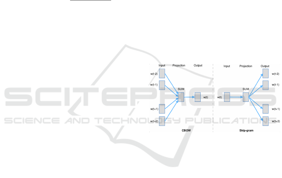
Word2vec implements two main learning algo-

rithms: CBoW (Continuous Bag of Words) and Skip-

gram (ﬁgure 1).

Figure 1: Simpliﬁed representation of the CBoW and Skip-

gram models (Mikolov et al., 2013).

CBoW is an architecture that predicts the current

word based on its surrounding context. Architecture

like Skip-gram does the opposite: it uses the current

word to predict surrounding words.

Building a Word2vec model is possible using

these two algorithms. The word order of the context

does not affect the result in any of these algorithms.

GloVe focuses on words co-occurrences over the

whole corpus. Its embeddings relate to the proba-

bilities that two words appear together. So, GloVe

combines features of Word2vec and singular co-

occurrence matrix decomposition.

In the present study, we applied both Word2vec

and GloVe models to obtain vector representations of

words.

The main application effect of using pre-trained

language models is to obtain high-quality vector rep-

resentations of words that take into account contex-

tual dependencies and allow you to achieve better re-

sults on targets.

Sentiment Analysis of Electronic Social Media Based on Deep Learning

167

4 DNNs Classiﬁcation Models

Design

After previous stage, we can start building a clas-

siﬁcation model. The model type and architec-

ture depends on the research task of SA which can

be performed at different hierarchical levels of text

documents (document-level, sentence-level, word or

aspect-level), domains (reviews about travel agencies,

hotels, movies, election opinion prediction, analysis

of public opinion on acute social and political issues),

binary or multiclass classiﬁcation.

If we have a dataset of texts with class labels

(for example, with binary labels “positive” and “neg-

ative”), we could apply Supervised ML techniques, in

particular, binary classiﬁcation algorithms.

Mathematically, this problem can be formulated

as follows: given training sample of texts X =

, x

, ...x

}, for each text there is a class label Y =

}, y

∈ {0, 1}, i = 1, 2, ...m.

It is necessary to build a classiﬁer model

b(X, w): X → Y , where w is a vector of unknown pa-

rameters or weights.

At the same time, it is necessary to minimize the

Loss function that determines the total deviation of

real class labels from those predicted by the classiﬁer.

For binary classiﬁcation problems, the most common

is binary cross-entropy:

Loss = −

∑

i=1

log(p

) + (1 − y

)log(1 − p

))

(4)

where N is the size of the training sample, y

= {0, 1}

is the true class label for the i-th data sample, p

is the

probability of belonging to the positive class for the

i-th data sample provided by the classiﬁer.

4.1 Logistic Regression

Since the task of SA in the general case is reduced to

the binary classiﬁcation problem (negative, positive),

we chose the Logistic Regression (LR) model as the

baseline classiﬁer b(·):

b(X, w) = σ (⟨w, x⟩), (5)

where ⟨w, x⟩ - denotes the scalar product, σ(·) is a

Sigmoid (logistic) function

σ(z) =

1 + exp(−z)

. (6)

LR has such advantage as it can be used to pre-

dict the probability to belong a training sample (in our

case, tokenized and vectorized text) to one of the two

target classes.

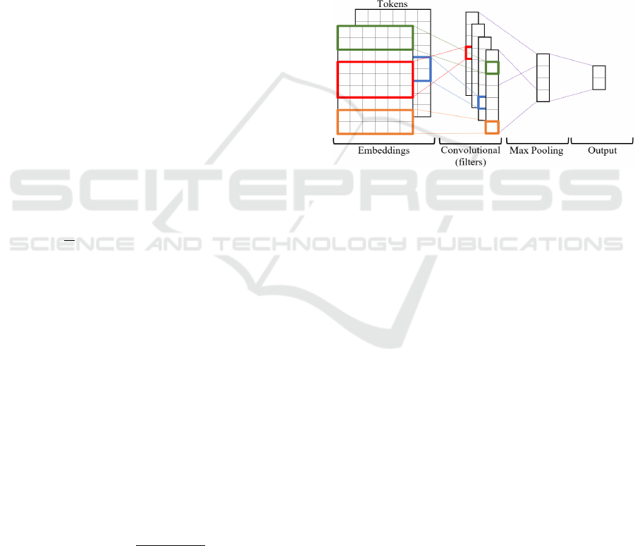
4.2 CNN Model

CNNs are a class of DNNs that were originally de-

signed for image processing (LeCun and Bengio,

1998). But these models have shown their efﬁciency

for many other tasks, such as time series forecasting

(LeCun et al., 2015).

Kim (Kim, 2014) has shown that CNNs are ef-

ﬁcient for classifying texts on different datasets. Re-

cently, they have also been used for various NLP tasks

(speech generation and recognition, text summariza-

tion, named entity extraction).

The architecture of CNNs consists of convolu-

tional and subsampling layers (ﬁgure 2).

Figure 2: Convolutional Neural Network (CNN) Architec-

ture for Text Processing (Kim, 2014).

The convolutional layer performs feature extrac-

tion from the input data and generates feature maps.

The feature map is computed through an element-

wise multiplication of the small matrix of weights

(kernel) and the matrix representation of the input

data, and the result is summed.

This weighted sum then passed through the

non-linear activation function. One of the most

common is the function ReLu, which is given as

ReLu(x) = max(0, x).

The pooling (subsampling) layer is a non-linear

compaction of the feature maps. For example, max-

pooling takes the largest element from the feature map

and extracts the sum of all its elements.

After max-pooling, feature maps are concatenated

into a ﬂatten vector, which will then be passed to a

fully connected layer.

The input data for the most NLP problems is text

which consists of sentences and words. So we need

represent the text as an array of vectors of a certain

length: each word mapped to a speciﬁc vector in a

vector space composed of the entire vocabulary.

As these vectors, we can use word frequencies

(for example, obtained using the T F − IDF metric),

or pre-trained embeddings (Word2vec, GloVe, Fast-

Text).

M3E2 2022 - International Conference on Monitoring, Modeling Management of Emergent Economy

168

Unlike images processing, text convolution is per-

formed using one-dimensional ﬁlters (1D Convolu-

tion) on one-dimensional input data, for example,

sentences, using convolution kernels of different size

(widths).

Applying of multiple kernels widths and feature

maps is analogous to the use of N-grams.

For image processing, convolutions are usually

performed on separate channels that correspond to the

colors of the image: red, green, blue. Set of different

ﬁlters is applied for each channel, and the result of

this operation is then merged into a single vector.

For text processing as channels we can consider,

for example, the sequence of words, or words embed-

dings. Then different kernels applied to the words can

be merged into a single vector.

The ﬁnal result of sentiment analysis is obtained

by applying Sigmoid activation function (binary clas-

siﬁcation task) or Softmax (in the case of multi-class

task).

4.3 LSTM and BiLSTM Model

Sequential information and long-term dependencies

in NLP traditionally performed with Recurrent Neu-

ral Networks (RNNs) which could compute context

information, for example, in dependency parsing.

The most common and efﬁcient for many ML

tasks, including NLP, were architectures based on

LSTM (Long Short Term Memory) or GRU (Gated

Recurrent Unit) cells (Brownlee, 2017; Kamath et al.,

2019).

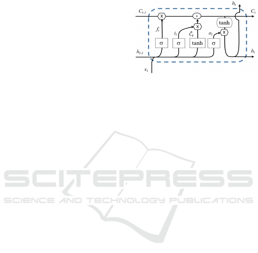
4.3.1 LSTM

LSTM model proposed by Hochreiter and Schmidhu-

ber (Hochreiter and Schmidhuber, 1997) introduces

the concept of a state for each of the layers of a RNN

which plays the role of memory.

The input signal affects the state of the memory,

and this, in turn, affects the output layer, just like in

a RNN. But this state of memory persists throughout

the time steps of a sequence (for example, time series,

sentence, or text document). Therefore, each input

signal affects the state of the memory as well as the

output signal of the hidden layer.

LSTM cell includes several units or gates: the in-

puts, output, and forget gates (ﬁgure 3). These gates

are used to control a memory cell that is carrying the

hidden state h

to the next time step.

The LSTM cell is formally deﬁned as:

= σ(W

· (h

t−1

, x

) + b

, (7)

= σ(W

· (h

t−1

, x

) + b

, (8)

Figure 3: Diagram of a LSTM cell.

= tanh(W

· (h

t−1

, x

) + b

), (9)

= σ(W

· (h

t−1

, x

) + b

), (10)

= i

⊗

, (11)

= f

⊗C

t−1

+ a

, (12)

where x

– is the vector of input sequence at time

t; C

t−1

, h

t−1

– state (long-term content) and hidden

state in previous time step (t − 1) respectively; σ(·),

tanh(·) are the Sigmoid and Hyperbolic tangent ac-

tivation functions; ⊗ – the Kronecker product; W

, W

– the weight matrices for input, forget, out-

put of the gates respectively; b

, b

– biases for the

gates.

The input gate i

determines which values need to

update. Then the hyperbolic tangent layer builds a

vector

of new values that can be added to the state

of the cell C

The forget gate f

controls how much is remem-

bered (what part of the information is kept and what

is erased) from step to step. Decision what informa-

tion can be thrown out of the cell state is made by a

sigmoid layer.

The output gate o

receives an input signal (which

is the concatenation of the input signal at time step

t and the cell output signal at time step (t − 1) and

passes it to the output. Thus, this gate determines

which part of the long-term content C

should be

transferred to the next time step.

Each of these gates is a feed-forward neural net-

work layer consisting of a sequence of weights ﬁtted

by the network with an activation function. This al-

lows the network to learn the conditions for forget-

ting, ignoring, or keeping information in the memory

cell.

Due its structure LSTM can learn and remember

representations for variable length sequences, such as

sentences, documents, and speech samples.

4.3.2 BiLSTM

Unidirectional (standard) LSTM only preserves in-

formation of the past because the only inputs it has

Sentiment Analysis of Electronic Social Media Based on Deep Learning

169

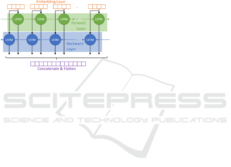
seen are from the past. Unlike standard LSTM, in

BiLSTM (Bidirectional LSTM) model the input ﬂows

in both directions and it’s capable of utilizing infor-

mation from both sides.

So BiLSTM is a sequence processing model that

consists of two LSTMs layers: one taking the input

in a forward direction (from “past to future”), and the

other in a backwards direction (from “future to past”)

(ﬁgure 4).

Figure 4: Diagram of a BiLSTM model.

For example, if we want to predict a word by

context (the central word), the network takes a given

number of words to the left of it as the context – the

Forward layer performs it, as well as the words to the

right of it – Backward layer performs it.

Then we can combine the outputs from both

LSTM layers in different ways: as sum, average, con-

catenation or multiplication. This output contains the

information or relation of past and future word.

BiLSTM increase the amount of information

available to the network, improving the context.

It’s also more powerful tool for modeling the se-

quential dependencies between words and phrases in

both directions of the sequence than standard LSTM.

BiLSTM is usually used when we have the se-

quence to sequence tasks but it should be noted that

BiLSTM (compared to LSTM) is a much “slower”

model and requires more time for training.

4.4 CNN+LSTM Model

Both basic DNNs architectures CNN and LSTM have

own advantages and disadvantages. Thus, LSTM net-

works can capture long-term dependencies and ﬁnd

hidden relationships in the data. CNNs are able to ex-

tract features using different convolutions and ﬁlters.

Therefore, the combination of convolutional and

recurrent layers in the model turns out to be effec-

tive in many applied problem such as simulation of

various natural processes, image processing, time se-

ries forecasting, and different NLP tasks (Chen and

Wang, 2018; Derbentsev et al., 2021; Islam et al.,

2020; Khan et al., 2022; Rasool et al., 2021; Shang

et al., 2020).

So we developed two models based on modiﬁ-

cations of CNN+LSTM architecture which ﬁnal de-

sign and hyperparameters settings are given in the

Section 6.

Our proposed models exploit the main features of

both LSTM and CNN. In fact, LSTM could accom-

modate long-term dependencies and overcome the

key issues with vanishing gradients. For this reason,

LSTM is used when longer sequences are used as in-

puts. On the other hand, CNN appears able to under-

stand local patterns and position-invariant features of

a text.

5 DATASETS AND SOFTWARE

IMPLEMENTATION

All developed DNNs (CNN, CNN-LSTM, BiLSTM-

CNN), and LR as the baseline, were implemented in

the Python 3.8 programming language using Scikit-

learn library for LR, estimation classiﬁcation accu-

racy, and for designing DNNs models we used Keras

library and TensorFlow as backend.

We evaluate the performance of our models on

two datasets: Stanford’s IMDb dataset (Stanford’s

Large Movie Review Dataset), which contains 50,000

movie reviews as well as Sentiment 140 dataset (Kag-

gle, 2022) with 1.6 million tweets.

Both datasets are intended for binary classiﬁca-

tion: they contain for each text (review or tweet) a

sentiment class binary label. They are also balanced,

i.e. contain the same number of texts for the positive

and negative classes.

6 EMPIRICAL RESULTS

6.1 Pre-Processing and Words

Embeddings

For text pre-processing the Python library package

NLTK (NLTK Project, 2022) was used, as well as cus-

tomers regular expressions.

The pre-processing stage included removing

punctuations, markup tags, html and tweet addresses,

removing stop words and converting all words to

lower case.

Tokenization was performed by using Keras pre-

processing text library. After tokenization we got the

length of the vocabulary in 92393 unique tokens for

M3E2 2022 - International Conference on Monitoring, Modeling Management of Emergent Economy

170

IMDb dataset and 507702 for Sentiment140 respec-

tively to which one token was added for representa-

tion out of vocabulary words.

It should be noted that the selected datasets are

characterized by different average length of texts

(number of words). Thus the length of most reviews

does not exceed 500 words, and tweets – 50.

Since DNNs work with ﬁxed-length input se-

quences we padded zero tokens all reviews and tweets

which length are less than average to ﬁxed length 500

and 50 words (tokens) respectively, and cut longer

texts to these ﬁxed sizes.

For words vector representation was used GloVe

word embeddings with word vectors of dimension

100 provided by Gensim library (

Reh

rek, 2022).

6.2 DNNs Models Design and

Hiperparameters Setting

To initialize the weights of the ﬁrst layer (Embedding

Layer) for all models, pre-trained GloVe embeddings

of size 100 were used. These weights were frozen and

did not change during training.

The ﬁrst model, CNN, consists of three sequential

Convolutional layers with ﬁlter sets of different ker-

nel widths. These layers are interspersed with Max-

pooling layers. Behind them are a Flatten and a Fully

connected (Dense) layer.

The second, CNN-LSTM model differs from the

CNN by the presence of an LSTM layer instead of

a Flatten after Convolutional and Maxpooling. The

base idea of such architecture is that CNN can be used

to retrieve higher-level word feature sequences and

LSTM to catch long-term correlations across window

feature sequences, respectively.

The third, BiLSTM-CNN model contains two

BiLSTM layers (forward and backward), followed by

a Convolutional and Maxpooling layers. After that,

two Fully connected layers were used to reduce the

output dimension and make prediction.

For all models Dropout layers were also used

to prevent overﬁtting. As the Loss-function Binary

Cross-Entropy (4) was chosen, which can be calcu-

lated as the average cross-entropy over all data sam-

ples (Geron, 2017).

The ﬁnal parameters of DNNs architecture are

shown in table 1.

6.3 Evaluating Performance Measures

The datasets were divided in the proportion of: 64%

for training, 20% for validation, and 16% for test sub-

sets respectively.

All DNNs models were trained over 5 epochs with

a minibatch size of 256 and 1024 samples for IMDb

and Sentiment 140 respectively. To compare classiﬁ-

cation performance of the developed models we used

the Accuracy metrics given by:

Accuracy =

T P + T N

P + N

× 100%, (13)

where T P and T N are the number of correctly pre-

dicted values of the positive and negative classes, re-

spectively; P and N are the actual number of values

for each of the classes.

We also calculated F1-score which is harmonic

average between Precision (the percentage of objects

in the positive class, which were classiﬁed as posi-

tive, are correctly classiﬁed), and Recall (percentage

of objects of the true positive class which we correctly

classiﬁed):

F1-score =

2T P

2T P + FP + FN

, (14)

Precision =

T P

T P + FP

, (15)

Recall =

T P

T P + FN

. (16)

Here FP (False Positive) and FN (False Negative) are

numbers of times (data samples) where the model in-

correctly classiﬁed these samples as belonging to the

positive and negative classes respectively.

The ﬁnal results of classiﬁcation performance are

presented in tables 2-3.

Classiﬁcation performance on IMDb dataset for

all developed DNN models is better than baseline.

The best Accuracy metric was obtained using the

CNN model (90.09%). At the same time, mod-

els based on the combination of Convolutional and

LSTM layers showed an Accuracy of 2-3% less

(table 2).

It should be noted that obtained results are compa-

rable or even superior in accuracy to the results given

by other researchers (Haque et al., 2020; Quraishi,

2020; Ali et al., 2019) for IMDb dataset.

All models showed signiﬁcantly lower accuracy

(on average 10% less) on the dataset Sentiment 140

(table 3). The best result was achieved for the

BiLSTM-CNN model – Accuracy 82.1%.

At the same time, the complication of models by

adding new layers did not lead to a signiﬁcant in-

crease in accuracy, but prolonged the training time.

In our opinion, lower accuracy may be due to the

fact that Sentiment 140 dataset contains many slang

words that are out of vocabulary. So, if for IMDb

dataset the part of the missing words was about 30

percent, then for the Sentiment 140 this part was more

than 70.

Sentiment Analysis of Electronic Social Media Based on Deep Learning

171

Table 1: Final DNNs models hyperparameters setting.

Model Layers Parameters

CNN Embedding emb dim 100, sent len 500(50)

Dropout 0.3

Convolutional 1D 100 ﬁlters of size 2, act func ReLu

Max pooling pool size 2

Convolutional 1D 100 ﬁlters of size 3, act func ReLu

Max pooling pool size 2

Convolutional 1D 100 ﬁlters of size 4, act func ReLu

Max pooling pool size 2

Flattent

Dropout 0.3

Fully connected 1 neuron, act func Sigmoid

CNN-LSTM Embedding emb dim 100, sent len 500(50)

Dropout 0.3

Convolutional 1D 50 ﬁlters of size 2, act func ReLu

Max pooling pool size 2

Convolutional 1D 100 ﬁlters of size 2, act func ReLu

Max pooling pool size 2

Convolutional 1D 200 ﬁlters of size 2, act func ReLu

Max pooling pool size 2

LSTM 64 neurons, reccur dropout 0.3

Dropout 0.3

Fully connected 32 neurons

Fully connected 1 neuron, act func Sigmoid

BiLSTM-CNN Embedding Emb dim 100, sent len 500(50)

Dropout 0.3

Bidirectional LSTM with 100 neurons

Dropout 0.3

Bidirectional LSTM with 100 neurons

Dropout 0.3

Convolutional 1D 100 ﬁlters of size 3, act func ReLu

Global Max pooling 1D

Fully connected 10 neurons, act func ReLu

Fully connected 1 neuron, act func Sigmoid

Table 2: Classiﬁcation performance on IMDb dataset,%.

Models Precision Recall F1-score Accuracy

LR (baseline) 86.62 85.54 86.08 85.90

CNN 90.04 90.31 90.18 90.09

CNN-LSTM 90.90 84.84 87.76 88.08

BiLSTM-CNN 83.08 93.25 87.87 87.03

Table 3: Classiﬁcation performance on Sentiment 140

dataset, %.

Models Precision Recall F1-score Accuracy

LR (baseline) 71.61 74.63 73.09 74.23

CNN 76.17 79.47 77.78 77.24

CNN-LSTM 78.98 77.47 78.23 78.37

BiLSTM-CNN 79.54 84.41 81.91 82.10

7 DISCUSSION AND

CONCLUDING REMARKS

Our research has shown that for sentiment analysis of

social media texts, at least for binary classiﬁcation,

DNNs of relatively simple architecture with a small

number of layers provide, in general, a level of accu-

racy acceptable enough for practical use.

For the selected English-language datasets IMDb

and Sentiment 140, the classiﬁcation accuracy using

the Logistic regression model (Baseline) was 85.9%

(74.23%), the CNN – 90.09% (77.24%), CNN-LSTM

– 88.01% (78.36%), and BiLSTM-CNN – 87.03%

(82.10%).

It should be noted that the accuracy of the clas-

siﬁcation can be increased if at the stage of pre-

M3E2 2022 - International Conference on Monitoring, Modeling Management of Emergent Economy

172

processing to execute lemmatization (or stemming)

which allow converting the words to their normal

form. This is especially true for tweets that contain

a large amount of user-generated vocabulary.

Also, it may be appropriate to use word embed-

dings weighted by their TF-IDF metric. It is also

possible for out of vocabulary words try to use the

weighted average value of the embeddings of the

neighboring words with a certain window length, or

replace the missing words with normalized TF-IDF

embeddings transformed using the principal compo-

nent method (SVD decomposition of the sparse TF-

IDF matrix to reduce its dimensionality).

In our opinion, a promising direction for carrying

out sentiment analysis of texts in social media is the

use of models based on deep convolutional networks,

or the synthesis of convolutional and recurrent net-

works, and applying the pre-trained embeddings (in

particular, based on GloVe, Word2vec, FastText mod-

els).

At the same time, the use of pre-trained embed-

dings allows to start learning DNNs not from ran-

domly generated values of model parameters, but al-

ready to some extent adapted to the task of text classi-

ﬁcation. Moreover, the learning process is accelerated

and the generalization abilities of classiﬁers based on

deep networks are improved.

REFERENCES

(2018). Natural Language Processing and Information Sys-

tems: Proceedings of 23rd International Conference

on Applications of Natural Language to Information

Systems, volume 10859 of Lecture Notes in Computer

Science. Springer Cham. https://doi.org/10.1007/

978-3-319-91947-8.

(2021). Soft Computing in Data Science 6th International

Conference, SCDS 2021, volume 1489 of SCDS: In-

ternational Conference on Soft Computing in Data

Science. Virtual Event, Springer, Singapore. https:

//doi.org/10.1007/978-981-16-7334-4.

Alessia, D., Ferri, F., Grifoni, P., and Guzzo, T. (2015). Ap-

proaches, tools and applications for sentiment analysis

implementation. International Journal of Computer

Applications, 125(3):26–33.

Ali, N. M., El Hamid, M. M. A., and Youssif, A. (2019).

Sentiment analysis for movies reviews dataset using

deep learning models. International Journal of Data

Mining & Knowledge Management Process (IJDKP),

9(2/3). https://aircconline.com/abstract/ijdkp/v9n3/

9319ijdkp02.html.

Bengio, Y., Ducharme, R., Vincent, P., and Jauvin, C.

(2003). A neural probabilistic language model. Jour-

nal of Machine Learning Research, 3:1137–1155.

https://proceedings.neurips.cc/paper/2000/ﬁle/

728f206c2a01bf572b5940d7d9a8fa4c-Paper.pdf.

Biesialska, M., Biesialska, K., and Rybinski, H. (2021).

Leveraging contextual embeddings and self-attention

neural networks with bi-attention for sentiment anal-

ysis. Journal of Intelligent Information Systems,

57:601–626. https://doi.org/10.1007/s10844-021-

00664-7.

Bojanowski, P., Grave, E., Joulin, A., and Mikolov, T.

(2017). Enriching Word Vectors with Subword In-

formation. Transactions of the Association for Com-

putational Linguistics, 5:135–146. https://doi.org/10.

1162/tacl a 00051.

Brownlee, J. (2017). Develop Deep Learning Models for

Natural Language in Python. Deep Learning for Nat-

ural Language Processing. http://ling.snu.ac.kr/class/

AI Agent/deep learning for nlp.pdf.

Camacho-Collados, J. and Pilehvar, M. T. (2018). On the

role of text preprocessing in neural network archi-

tectures: An evaluation study on text categorization

and sentiment analysis. In Proceedings of the 2018

EMNLP Workshop BlackboxNLP: Analyzing and In-

terpreting Neural Networks for NLP, pages 40–46,

Brussels, Belgium. Association for Computational

Linguistics. https://aclanthology.org/W18-5406.

Chen, N. and Wang, P. (2018). Advanced combined lstm-

cnn model for twitter sentiment analysis. In 2018

5th IEEE International Conference on Cloud Comput-

ing and Intelligence Systems (CCIS), pages 684–687.

https://doi.org/10.1109/CCIS.2018.8691381.

Deng, H., Ergu, D., Liu, F., Cai, Y., and Ma, B. (2022). Text

sentiment analysis of fusion model based on attention

mechanism. Procedia Computer Science, 199:741–

748. https://doi.org/10.1016/j.procs.2022.01.092.

Derbentsev, V., Bezkorovainyi, V., and Akhmedov, R.

(2020). Machine learning approach of analysis emo-

tion polarity electronic social media. Neiro-Nechitki

Tekhnolohii Modelyuvannya v Ekonomitsi, 9.

Derbentsev, V., Bezkorovainyi, V., Silchenko, M.,

Hrabariev, A., and Pomazun, O. (2021). Deep learning

approach for short-term forecasting trend movement

of stock indeces. In 2021 IEEE 8th International Con-

ference on Problems of Infocommunications, Science

and Technology (PIC S&T), pages 607–612. https:

//doi.org/10.1109/PICST54195.2021.9772235.

Devlin, J., Chang, M.-W., Lee, K., and Toutanova, K.

(2018). Bert: Pre-training of deep bidirectional trans-

formers for language understanding. https://arxiv.org/

abs/1810.04805.

Dhaoui, C., Webster, C. M., and Tan, L. P. (2017). So-

cial media sentiment analysis: lexicon versus machine

learning. Journal of Consumer Marketing, 34(6):480–

488. https://doi.org/10.1108/JCM-03-2017-2141.

Drus, Z. and Khalid, H. (2019). Sentiment analysis in so-

cial media and its application: Systematic literature

review. Procedia Computer Science, 161:707–714.

https://doi.org/10.1016/j.procs.2019.11.174.

Durairaj, A. K. and Chinnalagu, A. (2021). Transformer

based contextual model for sentiment analysis of cus-

tomer reviews: A ﬁne-tuned bert. International

Journal of Advanced Computer Science and Appli-

cations, 12(11). http://dx.doi.org/10.14569/IJACSA.

2021.0121153.

Sentiment Analysis of Electronic Social Media Based on Deep Learning

173

Elzayady, H., Mohamed, M. S., and Badran, S. (2021). Inte-

grated bidirectional lstm-cnn model for customers re-

views classiﬁcation. Journal of Engineering Science

and Military Technologies, 5(1). https://doi.org/10.

21608/EJMTC.2021.66626.1172.

Geetha, M. P. and Karthika Renuka, D. (2021). Improv-

ing the performance of aspect based sentiment anal-

ysis using ﬁne-tuned bert base uncased model. In-

ternational Journal of Intelligent Networks, 2:64–

69. https://www.sciencedirect.com/science/article/pii/

S2666603021000129.

Geron, A. (2017). Hands-On Machine Learning with Scikit-

Learn and TensorFlow. O’Reilly Media, Inc.

Haque, M. R., Salma, H., Lima, S. A., and Zaman, S. M.

(2020). Performance analysis of different neural net-

works for sentiment analysis on imdb movie reviews.

https://www.researchgate.net/publication/343046458.

Hern

andez, N., Batyrshin, I., and Sidorov, G. (2022). Eval-

uation of deep learning models for sentiment analysis.

Journal of Intelligent & Fuzzy Systems, pages 1–11.

https://doi.org/10.3233/JIFS-211909.

Hobson, L., Cole, H., and H.Hannes (2019). Natural Lan-

guage Processing in Action Understanding, analyz-

ing, and generating text with Python. Manning Publi-

cations.

Hochreiter, S. and Schmidhuber, J. (1997). Long Short-

Term Memory. Neural Computation, 9(8):1735–1780.

https://doi.org/10.1162/neco.1997.9.8.1735.

Iglesias, C. A. and Moreno, A., editors (2020). Sentiment

Analysis for Social Media. MDPI. https://doi.org/10.

3390/books978-3-03928-573-0.

Islam, M. Z., Islam, M. M., and Asraf, A. (2020). A

combined deep cnn-lstm network for the detection of

novel coronavirus (covid-19) using x-ray images. In-

formatics in Medicine Unlocked, 20:100412. https:

//doi.org/10.1016/j.imu.2020.100412.

Jain, P. K., Pamula, R., and Srivastava, G. (2021). A

systematic literature review on machine learning ap-

plications for consumer sentiment analysis using on-

line reviews. Computer Science Review, 41:100413.

https://doi.org/10.1016/j.cosrev.2021.100413.

Kaggle (2022). Sentiment140 dataset with 1.6 million

tweets. https://www.kaggle.com/datasets/kazanova/

sentiment140.

Kamath, U., Liu, J., and Whitaker, J. (2019). Deep Learn-

ing for NLP and Speech Recognition. Springer Cham.

https://doi.org/10.1007/978-3-030-14596-5.

Karamollao

glu, H., Do

gru,

I. A., D

orterler, M., Utku, A.,

and Yıldız, O. (2018). Sentiment analysis on turkish

social media shares through lexicon based approach.

In 2018 3rd International Conference on Computer

Science and Engineering (UBMK), pages 45–49.

https://ieeexplore.ieee.org/document/8566481.

Khan, L., Amjad, A., Afaq, K. M., and Chang, H.-T. (2022).

Deep sentiment analysis using cnn-lstm architecture

of english and roman urdu text shared in social me-

dia. Applied Sciences, 12(5):2694. https://doi.org/10.

3390/app12052694.

Khoo, C. S. and Johnkhan, S. B. (2018). Lexicon-

based sentiment analysis: Comparative evaluation

of six sentiment lexicons. Journal of Informa-

tion Science, 44(4):491–511. https://doi.org/10.1177/

0165551517703514.

Kim, Y. (2014). Convolutional neural networks for sentence

classiﬁcation. In Moschitti, A., Pang, B., and Daele-

mans, W., editors, Proceedings of the 2014 Confer-

ence on Empirical Methods in Natural Language Pro-

cessing, EMNLP 2014, October 25-29, 2014, Doha,

Qatar, A meeting of SIGDAT, a Special Interest Group

of the ACL, pages 1746–1751. ACL. https://doi.org/

10.3115/v1/d14-1181.

LeCun, Y. and Bengio, Y. (1998). Convolutional networks

for images, speech, and time series. In The Handbook

of Brain Theory and Neural Networks, page 255–258.

MIT Press, Cambridge, MA, USA.

LeCun, Y., Bengio, Y., and Hinton, G. (2015). Deep learn-

ing. Nature, 521(7553):436–444.

Li, H. (2017). Deep learning for natural language pro-

cessing: advantages and challenges. National Sci-

ence Review, 5(1):24–26. https://doi.org/10.1093/nsr/

nwx110.

Mayur, W., Annavarapu, C. S. R., and Chaitanya, K.

(2022). A survey on sentiment analysis meth-

ods, applications, and challenges. Artiﬁcial Intel-

ligence Review, 55:5731–5780. https://doi.org/10.

1007/s10462-022-10144-1.

Mikolov, T., Chen, K., Corrado, G., and Dean, J. (2013).

Efﬁcient estimation of word representations in vec-

tor space. In Bengio, Y. and LeCun, Y., editors,

1st International Conference on Learning Represen-

tations, ICLR 2013, Scottsdale, Arizona, USA, May

2-4, 2013, Workshop Track Proceedings. http://arxiv.

org/abs/1301.3781.

NLTK Project (2022). Natural language toolkit. https://

www.nltk.org/.

Pennington, J., Socher, R., and Manning, C. (2014). GloVe:

Global vectors for word representation. In Proceed-

ings of the 2014 Conference on Empirical Methods in

Natural Language Processing (EMNLP), pages 1532–

1543, Doha, Qatar. Association for Computational

Linguistics. https://aclanthology.org/D14-1162.

Pozzi, F., Fersini, E., Messina, E., and Liu, B. (2016). Sen-

timent Analysis in Social Networks. Elsevier Science.

Priyadarshini, I. and Cotton, C. (2021). A novel lstm–

cnn–grid search-based deep neural network for sen-

timent analysis. The Journal of Supercomput-

ing, 77(12):13911–13932. https://doi.org/10.1007/

s11227-021-03838-w.

Quraishi, A. H. (2020). Performance analysis of ma-

chine learning algorithms for movie review. Interna-

tional Journal of Computer Applications, 177(36):7–

10. https://doi.org/10.5120/ijca2020919839.

Rasool, A., Jiang, Q., Qu, Q., and Ji, C. (2021). Wrs:

A novel word-embedding method for real-time sen-

timent with integrated lstm-cnn model. In 2021

IEEE International Conference on Real-time Com-

puting and Robotics (RCAR), pages 590–595. https:

//doi.org/10.1109/RCAR52367.2021.9517671.

Reh

rek, R. (2022). Gensim: Topic modelling for humans.

https://radimrehurek.com/gensim/.

M3E2 2022 - International Conference on Monitoring, Modeling Management of Emergent Economy

174

Shang, L., Sui, L., Wang, S., and Zhang, D. (2020). Senti-

ment analysis of ﬁlm reviews based on CNN-BLSTM-

attention. Journal of Physics: Conference Series,

1550(3):032056. https://doi.org/10.1088/1742-6596/

1550/3/032056.

Sudhir, P. and Suresh, V. D. (2021). Comparative study

of various approaches, applications and classiﬁers

for sentiment analysis. Global Transitions Proceed-

ings, 2(2):205–211. https://www.sciencedirect.com/

science/article/pii/S2666285X21000327.

Tabinda Kokab, S., Asghar, S., and Naz, S. (2022).

Transformer-based deep learning models for the senti-

ment analysis of social media data. Array, 14:100157.

https://doi.org/10.1016/j.array.2022.100157.

Trisna, K. W. and Jie, H. J. (2022). Deep learning ap-

proach for aspect-based sentiment classiﬁcation: A

comparative review. Applied Artiﬁcial Intelligence,

36(1):2014186. https://doi.org/10.1080/08839514.

2021.2014186.

Sentiment Analysis of Electronic Social Media Based on Deep Learning

175