Analyze and Evaluate the Efficiency of the Tree-Based Process Scheduler

Ngo Hai Anh

1 a

and Ngo Dung Nga

2 b

Institute of Information Technology, Vietnam Academy of Science and Technology, Vietnam

International School, Vietnam National University, Hanoi, Vietnam

Keywords:

CFS, CPU Scheduling, FCFS, FIFO, Priority, Red-Black Tree, Round Robin, SJF.

Abstract:

In today’s computer systems, whether the programs execute on a single computer or on distributed systems,

scheduling plays a very important role in allocating system resources to processes. Our study analyzes some

common scheduling principles and focuses on evaluating the scheduling solution that is widely used in Linux–

based operating systems as a fair scheduling method, which was based on red–black tree data structure. Our

simulations was also conducted on a number of different sets of processes, to reflect real-world usage scenar-

ios.

1 INTRODUCTION

A process is a running program, or program in ex-

ecution. If the computer programs are not executed,

the main resource it consumes is only the amount of

memory, mainly the hard disk drive. But according

to the development of the computer hardware man-

ufacturing industry, the cost–per–unit of hard drive

is cheaper compared to other types of memory de-

vices such as registers, caches, or RAM (Toy and Zee,

1986). With modern computer systems, at the same

time there can be from a few dozen to hundreds of

processes running on individual machines as well as

thousands to tens of thousands of processes running

on distributed systems. An operating system (OS) is

software that acts as a resource manager, allocating

hardware resources appropriately to processes. When

a process is created, it receives the hardware resources

that the operating system allocates to it, including

CPU time, physical addresses on RAM, files on the

hard disk or input/output (I/O) devices (Bajaj1 et al.,

2015). In the operating system, scheduler will per-

form scheduling to efficiently allocate CPU time to

processes, in other words will switch CPU between

processes (Tanenbaum and Bos, 2015). Therefore, it

can be said that CPU scheduling is the basis for the

operation of multi-programming operating systems.

In this paper, we will analyze some popular schedul-

ing algorithms in the 2 section, then introduce a solu-

tion using advanced data structures for scheduling in

https://orcid.org/0000-0001-8982-0088

https://orcid.org/0000-0003-2774-3130

section 3. The next section 4 will simulate and evalu-

ate the proposed solution. And the last par t will be the

conclusion in section 5.

2 ANALYSIS OF SEVERAL

SCHEDULING METHODS

The simplest scheduling method is based on the prin-

ciple that process which first–come will be first–

served (means CPU time will be given first), called

the First-Come-First-Served (FCFS) algorithm, this

method uses a First-In First-Out (FIFO) data struc-

ture. Every time a process is created, it will be moved

to the queue and will have to wait for all the processes

already in the queue to finish executing (Adekunle

et al., 2014).

The different processes have different running

times, so scheduling by priority can also be applied.

Each process will be assigned a priority by the operat-

ing system, usually an integer number, and according

to the principle that the smaller number, the higher the

priority, and vice versa (Singh et al., 2014). A simple

variant of this priority-based method is the Shortest

Job First (SJF) algorithm, in which method, the pro-

cess with the shortest execution time will be allocated

CPU time by scheduler to run first, and so on for the

remaining processes with increasing execution time.

The two scheduling algorithms FIFO and Prior-

ity make sense in theory, but when implemented and

executed in the operating system, there can be prob-

lems, because processes have parameters very differ-

330

Anh, N. and Nga, N.

Analyze and Evaluate the Efﬁciency of the Tree-Based Process Scheduler.

DOI: 10.5220/0011924300003612

In Proceedings of the 3rd International Symposium on Automation, Information and Computing (ISAIC 2022), pages 330-335

ISBN: 978-989-758-622-4; ISSN: 2975-9463

 2023 by SCITEPRESS – Science and Technology Publications, Lda. Under CC license (CC BY-NC-ND 4.0)

ent: the time it is generated and passed to the sched-

uler to request the CPU – called arrival time, the time

it has to wait to be allocated the CPU – called wait-

ing time, and turnaround time is the time the process

is actually using the CPU to process its tasks. And

in fact, when users run computer programs, it is im-

possible to know in advance when the process will

pause, stop (close) because that completely depends

on user behavior. Therefore a scheduling method of

rotation type (called Round Robin–RR) can be ap-

plied. The idea of this approach is that each process

will be given a fixed amount of time by the operat-

ing system q called quantum. Ideally, q is enough or

more than enough for the process to finish its task,

otherwise the process is forced to stop using the CPU

after the q interval and wait for the next CPU run, and

the next running turns are allocated CPU time up to q

(time unit) (Rajput and Gupta, 2012; Shyam and Nan-

dal, 2014).

If there are n processes in the queue waiting for

their turn to execute, the RR algorithm will not care

about queue order or priority like the FCFS/FIFO

or Priority algorithms as above, it will distribute to

each process 1/n of CPU time and each distribution

does not exceed the q quota. No process has to wait

more than q(n− 1) (CPU time). In fact, operating sys-

tems often choose the value of q in the range 1–10

(ms) (Tanenbaum and Bos, 2015).

To see the difference between the above algo-

rithms, let us consider an example as follows: sup-

pose there are five processes P

, and P

are

open and pending (granted CPU time) respectively.

Assume the time required for processes to complete

their tasks is 10, 6, 2, 4, and 8 (ms) respectively;

The priority for each process is 3, 5, 2, 1, and 4

respectively (the higher the priority, the higher the

priority). We will evaluate the criterion turnaround

time–which is the average actual running time (CPU

usage) of the five processes mentioned above. With

the FCFS algorithm, the scheduler will run in the or-

der P

→ P

. P

runs for 10ms, P

runs for 16ms (because it has to wait for P

to fin-

ish), just like that we can calculate P

which takes

18ms, P

took 22ms and P

took 30ms. The average

turnaround time for all five processes to complete is

19.2ms. With the Priority algorithm, the running or-

der is P

→ P

. P

runs for 6ms,

runs for 14ms (because we have to wait for P

to finish), just like that we can calculate P

which

takes 18ms, P

took 22ms and P

took 30ms. The av-

erage turnaround time with this algorithm is 18ms.

With the RR algorithm, the running order of the pro-

cesses doesn’t matter, each P

will in turn take up 1/5

of the CPU time, and so on until the first process ter-

minates (which is P

)

.3), then each remaining process

is given 1/4 CPU in turn, and so on until the end, the

total turnaround time (running time) of these five pro-

cesses is (10 + 18 + 24 + 28 + 30) = 110ms, average

is 22ms.

Thus, it can be seen that the RR algorithm has a

longer running time than the two FCFS/FIFO and Pri-

ority algorithms, but this algorithm has the advantage

of evenly distributing the CPU usage limit for the pro-

cesses, which is quite important. This is important be-

cause in practice the schedulers in the operating sys-

tem will not know in advance when the user will open

the program, how long the open program will run,

or when the user will stop the running program. In

essence, the data structure used by RR is still in the

form of FIFO and still has processes that reserve the

right to run first (in the above example P

), but can

only run within the CPU allocation limit (above is 1/5

when all five processes have not finished running, and

increments from 1/4–1 each time one, two, three and

four processes terminate) (Noon et al., 2011).

3 ANALYSIS OF SCHEDULING

IMPROVED SOLUTIONS

BASED ON TREE DATA

STRUCTURES

With the analysis of some scheduling algorithms as

mentioned above, we see that these algorithms still

depends on the fixed priority value or equally divided

resources among the processes, so when installed in

the operating systems, it is possible to use uses binary

tree data structures and some improved data structures

from binary trees, such as Heap (Gabriel et al., 2016).

These algorithms based on binary tree data structures

have been proven to have a complexity of O(1) or

O(N) (Aas, ).

With built-in in the Linux kernel since version 2.4,

the O(N) scheduler uses the O(N) algorithm, where

the execution time is a function of the number of pro-

cesses, here is N. Or more accurately, the time of the

algorithm is a linear function of N, i.e. as N increases,

the time increases linearly. Scheduler O(N) can termi-

nate if N is continuously increasing. This scheduling

method is simple but will have poor performance on

systems running multiple CPUs (multiprocessors) or

multiple cores.

The O(1) scheduler, running in constant time as

the name suggests, has been integrated into the Linux

kernel since version 2.4, no matter how many pro-

cesses are running in the system, this scheduler can

guaranteed to finish in a fixed time. This makes O(1)

Analyze and Evaluate the Efﬁciency of the Tree-Based Process Scheduler

331

scale better than O(N) relative to the number of pro-

cesses, thus solving the performance problems of

O(N).

In general, the O(1) scheduler uses a priority-

based scheduling policy. The scheduler chooses the

most appropriate process to run based on their pri-

ority. The O(1) scheduler is the multi-queues sched-

uler. The main structure of the O(1) scheduler is two

runqueue queues, one active and one expired. The

Linux kernel can access these two queues via pointers

on each CPU, which can be swapped with a swapping

pointer.

On modern computing systems such as personal

computers, mobile devices,. . . applications that are of-

ten highly interactive or run in real time, an important

property that needs to be ensured is fairness, fairness

to processes means that when scheduled by the oper-

ating system, they must have a fair share in process-

ing time. Therefore, the queue structure also needs

to be changed to ensure compliance with a Com-

pletely Fair Scheduler (Jones, 2022). red–black tree–

rbt (Bayer, 1972; Guibas and Sedgewick, 1978) is a

self-balancing binary search tree. Each node of a red-

black tree has a property “color” that takes either the

value red or black and the following properties:

• A node is either red or black;

• Root and leaf nodes (leaf nodes with NULL value)

are black;

• The children of every red node are black, i.e. every

red node whose parent node is black;

• All paths from any node to leaves have the same

number of black nodes.

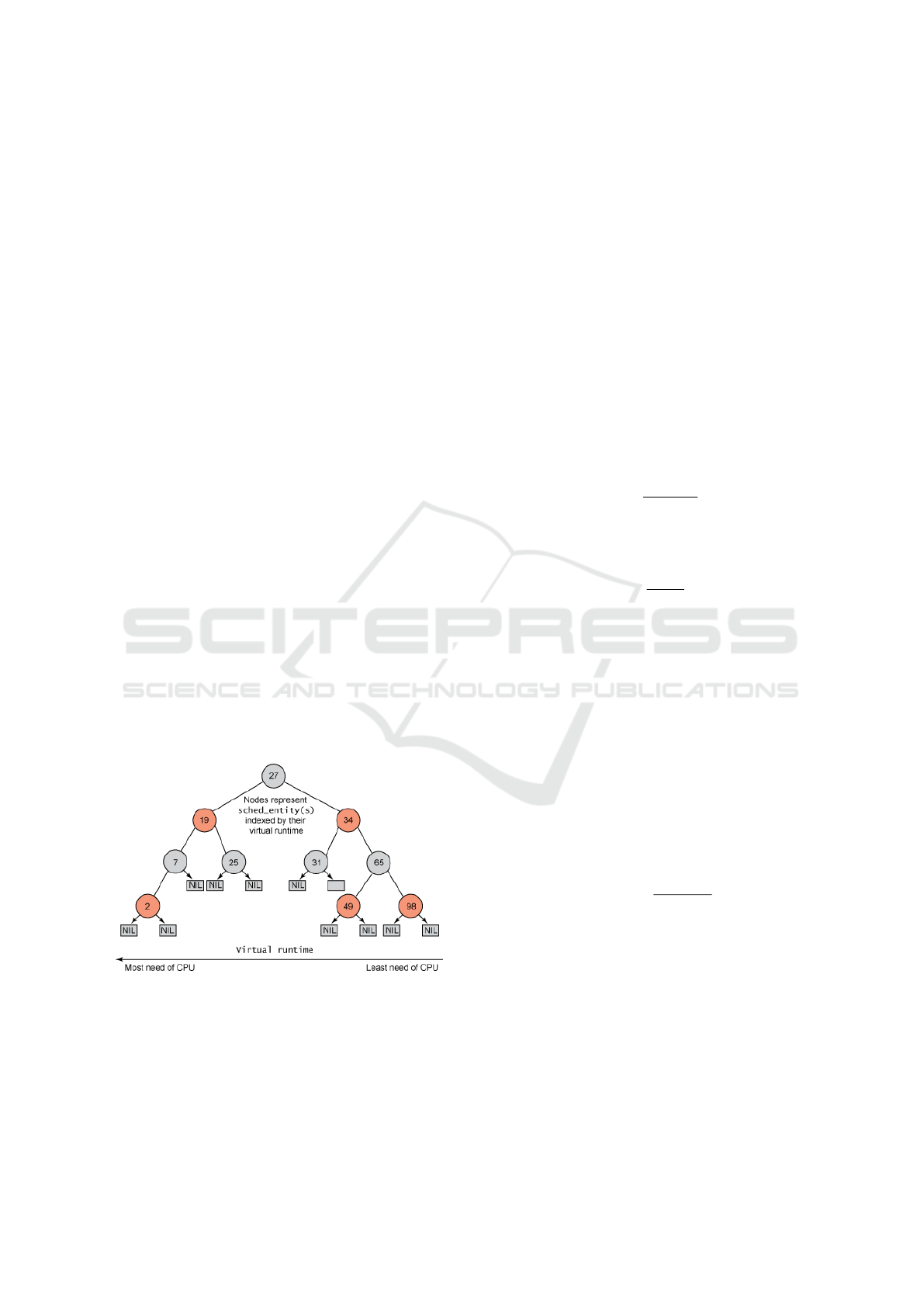
Figure 1: The red–black tree used to represent the pro-

cesses (Jones, 2022).

The red–black tree has many useful properties.

First, to search in the red–black tree will take O(logn)

time. Second, it is self–balancing, which means that

no path in a tree is twice as long as any other. So, in

a rbt tree as shown in figure 1, every node represents

a process (or task) in the system, and the node’s key

value represents runtime of this particular task. With

the definition of red-black tree means, the leftmost

node has the smallest key value, which means this task

has the smallest virtual runtime, so this task needs

the most processing. On the other hand, the rightmost

node has the largest key value, which means this task

is the least necessary to be executed. So the scheduler

simply selects the leftmost task for the processor. Af-

ter the leftmost task is processed, it is removed from

the tree. Since this task already has some processing

time, its virtual runtime is increased. And then, if this

task is not completed, it will be inserted back into the

red–black tree with the new virtual runtime. And the

time for this operation is O(logn).

We will calculate the vruntime of the processes

in the figure 1 in the following steps. First need to

calculate LWT (Load Weight Ratio):

LWT

∑

i=1

(1)

In the formula 1 LW

is the Load Weight of each

process, and is calculated by the formula:

1024

1.25

(2)

here, P

is the priority assigned to the processes. In

operating systems like Linux, this integer value P

is called nice_value and ranges from {-20, 19}, the

smaller the value, the higher the precedence.

Based on the formulas 1 and 2 we can calculate

the running time vruntime of the processes in the red-

black tree over a period of time p as follows:

vruntime

= LW T

× p (3)

here, the minimum value of p is 20ms in Linux oper-

ating system.

To check the fairness of dividing the p time inter-

val for processes based on the tree structure rbt in the

formula 3, we give the following formula:

f airness

LWT

× p

(4)

In Table 1 we see the running time vruntime of

different priority processes in the observation period

p = 100ms. The red–black tree–based scheduling al-

gorithm rbt first converts the payload LW

of the pro-

cesses i based on the pr iority value P initial set by

the operating system, from which the corresponding

load ratio LW T

and then the running time vruntime,

all these runtimes are different, but they all have the

same f airness.

ISAIC 2022 - International Symposium on Automation, Information and Computing

332

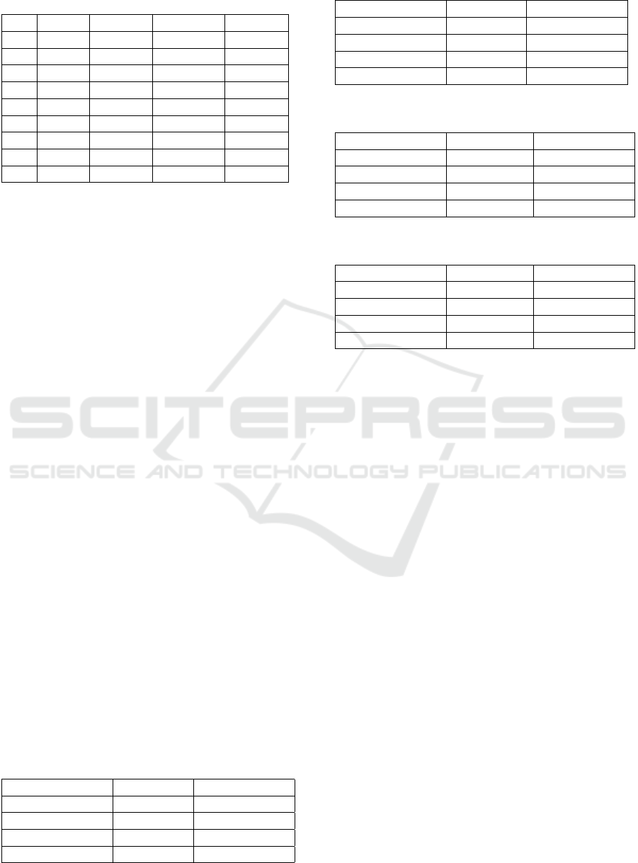
Table 1: Fairness by scheduling algorithm based on red-

black tree structure rbt.

P LW LWT vruntime fairness

-20 88818 0.67233 67.23343 0.77515

-15 29104 0.22031 22.03105 0.77515

-10 9537 0.07219 7.21913 0.77515

-5 3125 0.02366 2.36557 0.77515

0 1024 0.00775 0.77515 0.77515

5 336 0.00254 0.25400 0.77515

10 110 0.00083 0.08323 0.77515

15 36 0.00027 0.02727 0.77515

19 15 0.00011 0.01117 0.77515

4 SIMULATION AND RESULTS

ANALYZING

4.1 Comparison of Scheduling Using

Red-Black Trees and Heap Trees

To evaluate the efficiency of the fair scheduling algo-

rithm based on the red–black tree structure rbt. We

compare with the binary tree–based scheduling algo-

rithm Heap as analyzed in Section 3. The compari-

son was made on four scenarios of increasing num-

ber of processes: from 100–for a personal computer or

mobile device; 1000–suitable for a powerful personal

computer; 10000–corresponds to a server providing

basic services such as web or email, and finally 20000

processes–equivalent to a server providing distributed

services, cloud. . . For each scenario, we compare the

following criteria:

1. Algorithm running time (how long the scheduler

takes to finish processing)

2. Average waiting time of processes, this is the time

each process P

waits until it receives CPU time.

3. Average turnaround time of processes, this is the

time that P

processes occupy the CPU, i.e. are be-

ing processed

4. Throughput (is the number of processes that can

run in a unit of time)

With the above criteria, the better algorithm will have

less time and more throughput. Tables 2, 3, 4 and 5

aggregates the results of the four suggested scenarios.

Table 2: 100–process scenario.

Criteria Heap tree Red-Black tree

Running time 10 062 200 3 026 900

Waiting time 3 723 380 1 119 670

Turnaround time 3 826 558 1 150 697

Throughput 9.94 33.04

Table 3: 1000–process scenario.

Criteria Heap tree Red-Black tree

Running time 86 487 000 76 853 300

Waiting time 42 679 490 37 954 810

Turnaround time 42 765 926 38 031 670

Throughput 11.56 13.01

Table 4: 10000–process scenario.

Criteria Heap tree Red-Black tree

Running time 193 085 900 76 853 300

Waiting time 98 245 584 58 437 288

Turnaround time 98 264 862 58 448 754

Throughput 51.79 86.86

Table 5: 20000–process scenario.

Criteria Heap tree Red-Black tree

Running time 343 634 700 278 669 000

Waiting time 169 744 048 137 299 910

Turnaround time 169 761 184 137 313 770

Throughput 58.21 71.77

In the four result tables above, the time values are

in nanoseconds (10

−9

s) because modern processors

are all in this range, while the throughput is in the

number of tasks the scheduler can handle per millisec -

ond (10

−3

s) because ms is the right amount of time for

the CPU to divide among the processes. All four pro-

posed simulation scenarios show a much better perfor-

mance of the fair scheduling algorithm based on the

red–black tree than the priority scheduling algorithm

based on the Heap binary tree.

Looking at the results we also see that in the sce-

nario 3 with the number of processes about 1000,

equivalent to a good personal computer, there is a

slight difference in the performance of both schedul-

ing types. As for systems with few or many processes

(in scenarios 2, 4 and 5), the difference in processing

time as well as processing capacity is much larger, and

the fairness scheduler using the red–black tree proved

to be more advantage, this is very important because

nowadays the trend of using compact personal devices

such as smartphones, or large computing systems ac-

cording to distributed, cloud, edge, fog,. . . computing

models becomes popular, the proportion of personal

computers tends to decrease. That said, scheduling

algorithms suitable for such devices would has very

high practical significance.

Analyze and Evaluate the Efﬁciency of the Tree-Based Process Scheduler

333

4.2 Comparison of Scheduling

Algorithms Using Red-Black Trees

and FIFO, Round Robin and

Multi-Level

To evaluate the efficiency of the fair scheduling al-

gorithm based on the red–black tree structure rbt

with traditional algorithms such as FCFS, SJF, Round

Robin mentioned in 2 and a algorithm we propose

consisting of many levels that combine these algo-

rithms in a queue called Multi-Level Queue as below:

• Level 1: Round Robin with q = 3, used for priority

0, 1 (high priority)

• Level 2: Round Robin with q = 5, used for priority

levels 2, 3 (low priority)

• Level 3: FCFS, used for lowest priority.

The reason for choosing the combination of the above

algorithms is as follows: we find that with low pri-

ority, the process will be executed on a first–come,

first–served method, with processes with lower prior-

ity. Higher priority needs to avoid CPU occupation, so

Round Robin algorithm will be applied with the quan-

tum q = 5, and for processes with higher priority, it is

necessary to further reduce the quantum q = 3. Such a

combination will ensure more fairness than applying

a single algorithm for CPU allocation to processes.

We compare the performance of the algorithms

according to two criteria, waiting time and turnaround

time applied on the same four scenarios as in sec-

tion 4.1 (100, 1000, 10000 and 20000 randomly gen-

erated processes).

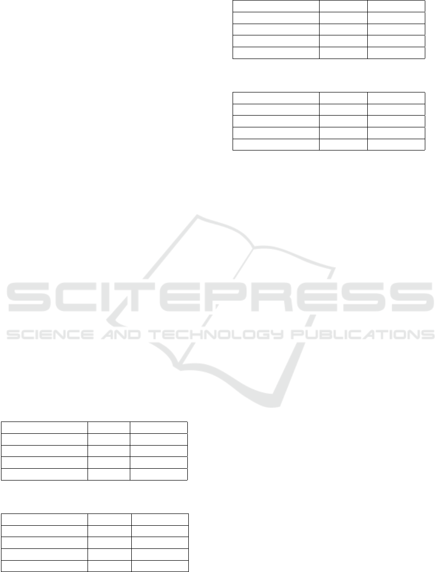
Tables 6, 7, 8 and 9 aggregates the results of the

four proposed scenarios. Time is calculated as the av-

erage of all processes in each scenario.

Table 6: 100-processes scenario.

Algorithm Waiting Turnaround

FCFS 252.93 258.50

Round Robin 325.68 331.25

Multi-Level Queue 251.08 256.65

Red-Black Tree 223.70 229.27

Table 7: 1000-processes scenario.

Algorithm Waiting Turnaround

FCFS 2434.95 2440.29

Round Robin 3165.29 3170.64

Multi-Level Queue 2499.27 2504.62

Red-Black Tree 2150.95 2156.27

Table 8: 10000-processes scenario.

Algorithm Waiting Turnaround

FCFS 24912.09 24917.59

Round Robin 32620.82 32626.32

Multi-Level Queue 25514.42 25519.92

Red-Black Tree 22647.70 22653.20

Table 9: 20000-processes scenario.

Algorithm Waiting Turnaround

FCFS 49842.19 49847.68

Round Robin 65063.31 65068.80

Multi-Level Queue 51268.53 51274.02

Red-Black Tree 45126.44 45131.93

Look at the simulation results in the tables 6, 7, 8

and 9 we see that for as few processes as in the

tables 6, 7 (the actual equivalent of the number

of prog rams running on a mobile device, or high-

end personal computer) the scheduling methods do

not make a big difference, however scheduling us-

ing a red–black tree still gives the best results, round

robin scheduling for the longest time is understand-

able given the sequential nature of resource alloca-

tion (requirements are met in turn) of Round Robin.

With a large number of processes as shown in the ta-

bles 8 and 9 the difference between the algorithms is

shown clearer, and scheduling using red–black trees

still guarantees the best results.

5 CONCLUSIONS

Process scheduling or in other words determining the

runtime for programs on a computer system is a very

important issue because the nature of computer sys-

tems is to share hardware resources, especially with

division or allocation of time using the CPU, where

execution time is calculated in CPU cycles with nano–

second latency. Priority–based scheduling methods

often assign different priorities to processes, these pri-

orities are usually fixed, the implementation of such

algorithms is often based on a binary tree structure.

With applications that increasingly require very high

interaction with users as well as between devices,

it is necessary to have a scheduler that provides a

fair distribution of resources between processes. Fair

scheduling method using red–black tree data structure

has many advantages in ensuring fairness between

processes. Our research has focused on analyzing this

fair scheduling method, with some parameters consid-

ered on Linux operating system. The analysis results

are evaluated based on the process sets with different

numbers suitable for current computer systems, and

ISAIC 2022 - International Symposium on Automation, Information and Computing

334

all show the advantages of the fair scheduling algo-

rithm using the tree data structure, red–black com-

pared to traditional algorithms that use simpler data

structures such as FIFO, Round Robin, or by prior-

ity. However, if the FIFO or Round Robin algorithms

are properly combined, the performance can still be

roughly equivalent to fair scheduling using a red–

black tree data structure.

ACKNOWLEDGEMENTS

This work was supported by the Vietnam Academy

of Science and Technology (grant number

VAST01.09/22-23).

REFERENCES

Aas, J. Understanding the Linux 2.6.8.1 CPU Scheduler.

Accessed: 2021-08-19.

Adekunle, Y., Ogunwobi, Z., Jerry, A. S., Efuwape, B.,

Ebiesuwa, S., and Ainam, J.-P. (2014). A Comparative

Study of Scheduling Algorithms for Multiprogram-

ming in Real-Time Systems. International Journal of

Innovation and Scientific Research, 12:180–185.

Bajaj1, C., Dogra, A., and Singh, G. (2015). Review And

Analysis Of Task Scheduling Algorithms. Interna-

tional Research Journal of Engineering and Technol-

ogy (IRJET), 02:1449–1452.

Bayer, R. (1972). Symmetric Binary B-Trees: Data

Structure and Maintenance Algorithms. Acta Inf.,

1(4):290–306.

Gabriel, P. H., Albertini, M. K., Castelo, A., and de Mello,

R. F. (2016). Min-heap-based scheduling algorithm:

an approximation algorithm for homogeneous and het-

erogeneous distributed systems. International Jour-

nal of Parallel, Emergent and Distributed Systems,

31(1):64–84.

Guibas, L. J. and Sedgewick, R. (1978). A dichromatic

framework for balanced trees. In 19th Annual Sympo-

sium on Foundations of Computer Science (sfcs 1978),

pages 8–21.

Jones, M. T. (2018 (accessed October 10, 2022)). Inside the

linux 2.6 completely fair scheduler. https://developer.

ibm.com/tutorials/l-completely- fair-scheduler/.

Noon, A., Kalakech, A., and Kadry, S. (2011). A New

Round Robin Based Scheduling Algorithm for Operat-

ing Systems: Dynamic Quantum Using the Mean Av-

erage. International Journal of Computer Science Is-

sues, 8.

Rajput, I. S. and Gupta, D. (2012). A Priority based Round

Robin CPU Scheduling Algorithm for Real Time Sys-

tems. International Journal of Innovations in Engi-

neering and Technology, 01(3):1–11.

Shyam, R. and Nandal, S. K. (2014). Improved Mean Round

Robin with Shortest Job First Scheduling. Interna-

tional Journal of Advanced Research in Computer Sci-

ence and Software Engineering, 04(7):170–179.

Singh, P., Singh, V., and Pandey, A. (2014). Analysis and

Comparison of CPU Scheduling Algorithms. Interna-

tional Journal of Emerging Technology and Advanced

Engineering, 04(1):91–95.

Tanenbaum, A. and Bos, H. (2015). Modern Operating Sys-

tems, 4th Edition. Pearson Higher Education.

Toy, W. N. and Zee, B. (1986). Computer Hardware-

Software Architecture. Prentice Hall Professional

Technical Reference.

Analyze and Evaluate the Efﬁciency of the Tree-Based Process Scheduler

335