3D Transient CFD Modelling of a Museum Showcase with

Environmental Air Exchange

Na He

, Heng Yi

, Quan Yuan and Zheren Jiang

Chongqing China Three Gorges Museum, Chongqing, China

Keywords: CFD, Transient Analysis, Museum Showcase, Air Exchange Rate.

Abstract: A 3D transient CFD model is established to characterize heat and mass transfer phenomena in a museum

showcase with environmental air exchange in Chongqing China Three Gorges Museum. The model is able to

give detailed information about air temperature and velocity distributions in the showcase at different time

points during the periods investigated. In order to evaluate the model’s accuracy, experiments are performed

in two typical days in summer and winter, while the temperature variation data is collected. The model is

validated with the experimental data and shows satisfactory accuracy with average deviation within 0.1°C. A

numerical method to calculate air exchange rate (AER) of museum showcases with environmental air

exchange is proposed for as an application of this model. The method simulates the carbon dioxide tracer

dilution process in the showcase, and the simulated tracer concentration curves are used to calculate the air

exchange rate of the showcase successfully. Calculation results in both cases show that AERs increase with

environmental temperature. This work proves CFD to be a powerful tool in the modelling of museum

showcases.

1 INTRODUCTION

Preventive conservation is a significant methodology

for long-term preservation of cultural heritage(Getty

Institute, 1994). The key thought of preventive

conservation is to protect cultural heritage from the

environmental risks(Kissel, 1999). Environmental

risks are determined by parameters including air

quality, temperature and humidity, so monitoring and

controlling of these parameters are significant tasks

of preventive conservation(Ankersmit & Stappers,

2017). Museum showcases are significant preserving

and displaying facilities for the cultural heritage in

museums, so the effects of showcases on the

preserving environmental parameters should be

carefully evaluated, which makes a performance

model for the showcases significant. A parametric

model has been proposed to characterize air exchange

performance of museum showcases with a single

parameter, i.e. air exchange rate (AER)(Thomson,

1977). However, the one-parameter model is not

enough to give detailed description of the coupled air

flow, heat transfer and mass transfer phenomena in

https://orcid.org/0000-0002-0798-5709

https://orcid.org/0000-0002-8393-396X

3D space. Recently, researchers started to apply

computational fluid dynamics (CFD) to the modelling

of museum showcases. CFD can visualize in detail

the physical process occurring in the museum

showcases, thus can help with their design and

optimization(Liu et al., 2008; Wang et al., 2013.).

CFD is a type of computer aided engineering tool

capable of describing fluid flow, heat transfer and

mass transfer processes. It is widely used in various

fields such as aerospace, automotive and building

ventilation(Peng et al., 2016; Xia et al., 2010; Yi et

al., 2021). Some researchers attempted to apply CFD

methods to the field of cultural heritage preservation,

especially the preservation of some historic

buildings(Balocco et al., 2014; D’Agostino et al.,

2014; D’Agostino & Congedo, 2014; Oetelaar, 2016;

Pasquarella et al., 2013). For example, D'Agostino et

al. applied CFD to describe the airflow and salt

crystallization process in a historical church in

Italy(D’Agostino et al., 2014; D’Agostino &

Congedo, 2014). Oetelaar applied CFD to simulate

the thermal environment inside a set of ancient

Roman baths(Oetelaar, 2016). Balocco et al. applied

310

He, N., Yi, H., Yuan, Q. and Jiang, Z.

3D Transient CFD Modelling of a Museum Showcase with Environmental Air Exchange.

DOI: 10.5220/0011923900003612

In Proceedings of the 3rd Inter national Symposium on Automation, Information and Computing (ISAIC 2022), pages 310-317

ISBN: 978-989-758-622-4; ISSN: 2975-9463

 2023 by SCITEPRESS – Science and Technology Publications, Lda. Under CC license (CC BY-NC-ND 4.0)

CFD to simulate the heat and moisture transfer

process in a historical library room with people

movements considered(Balocco et al., 2014;

Pasquarella et al., 2013). Nevertheless, only a few

studies applied CFD to the modeling and analysis of

museum showcases. Wang(Wang et al., n.d.) applied

CFD to simulate the air temperature and flow velocity

distributions in two showcases with lamps as heat

sources. Different air exchange flowrates were

imposed to investigate the effects, while the heat

transfer between the showcases and the environment

was not taken into account. Liu(Liu et al., 2008) built

a 2D CFD model to simulate the heat transfer between

the showcase and the environment under summer and

winter conditions. Constant environment

temperatures were imposed in the model, while real-

time temperature variation during the days was not

taken into account.

Although the studies above applied CFD to model

museum showcases, they all adopted major

simplifications to the models which limited scope of

the models’ applications. The modelling method

could be further improved if the following two

aspects are taken into account. Firstly, real-time

transient temperature variation needs to be imposed

to the model, so that the simulation results are

comparable to the experimental data, which makes

the experimental validation of the model possible.

Secondly, the coupled air flow, heat transfer and mass

transfer process needs to be taken into account for the

museum showcases as well as the environment. With

the points above taken into account, this work is

dedicated to build and validate a 3D transient CFD

model for a museum showcase with varied

environmental temperature imposed, while the air

exchange between the showcase and environment is

modelled simultaneously.

To be specific, the following key points are

discussed in this paper:

1) The 3D CFD model with transient

environmental conditions is established for a museum

showcase with environmental air exchange.

2) Experiments are performed for the showcase in

two typical days in summer and winter.

3) The model is validated with the experimental

temperature data and the accuracy is evaluated.

4) The validated model is applied to calculate the

air exchange rate of the showcase in summer and

winter.

2 EXPERIMENTAL SETUP

2.1 The Showcase

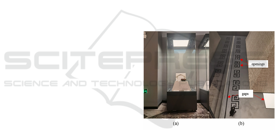
The museum showcase investigated is located in the

Chongqing China Three Gorges Museum, and is

shown in Figure 1(a). The showcase consists of three

parts: the upper part which is an aluminium box with

a set of lamps installed, the middle part made of glass

in which the artifacts are preserved and displayed, and

the bottom part made of aluminium sheet which acts

as base of the showcase. A wooden table is placed in

the middle part on which the artifacts are displayed.

It should be noted that there are 18 openings and two

gaps at bottom of the middle part as shown in Figure

1(b). The showcase is well sealed except for the

openings and gaps mentioned above which connect

the air inside to the environment. There is no

individual temperature control and ventilation system

for this showcase, so the temperature distribution

inside is indirectly determined by surrounding

environment.

Figure 1: The museum showcase: (a) Overall structure; (b)

Openings and gaps in the middle part.

2.2 Monitoring Device

The monitoring device in this work consists of seven

Testo 160TH sensors which can measure and record

parameters including temperature and humidity. One

sensor (sensor A in Figure 2) is placed inside the

showcase to measure the temperature inside. The

other six sensors (sensors B, C, D, E, F, and G in

Figure 2) are placed outside the showcase to record

the environmental temperature. The temperatures are

recorded every 1 minute for sensor A and every 15

minutes for the other six sensors.

3D Transient CFD Modelling of a Museum Showcase with Environmental Air Exchange

311

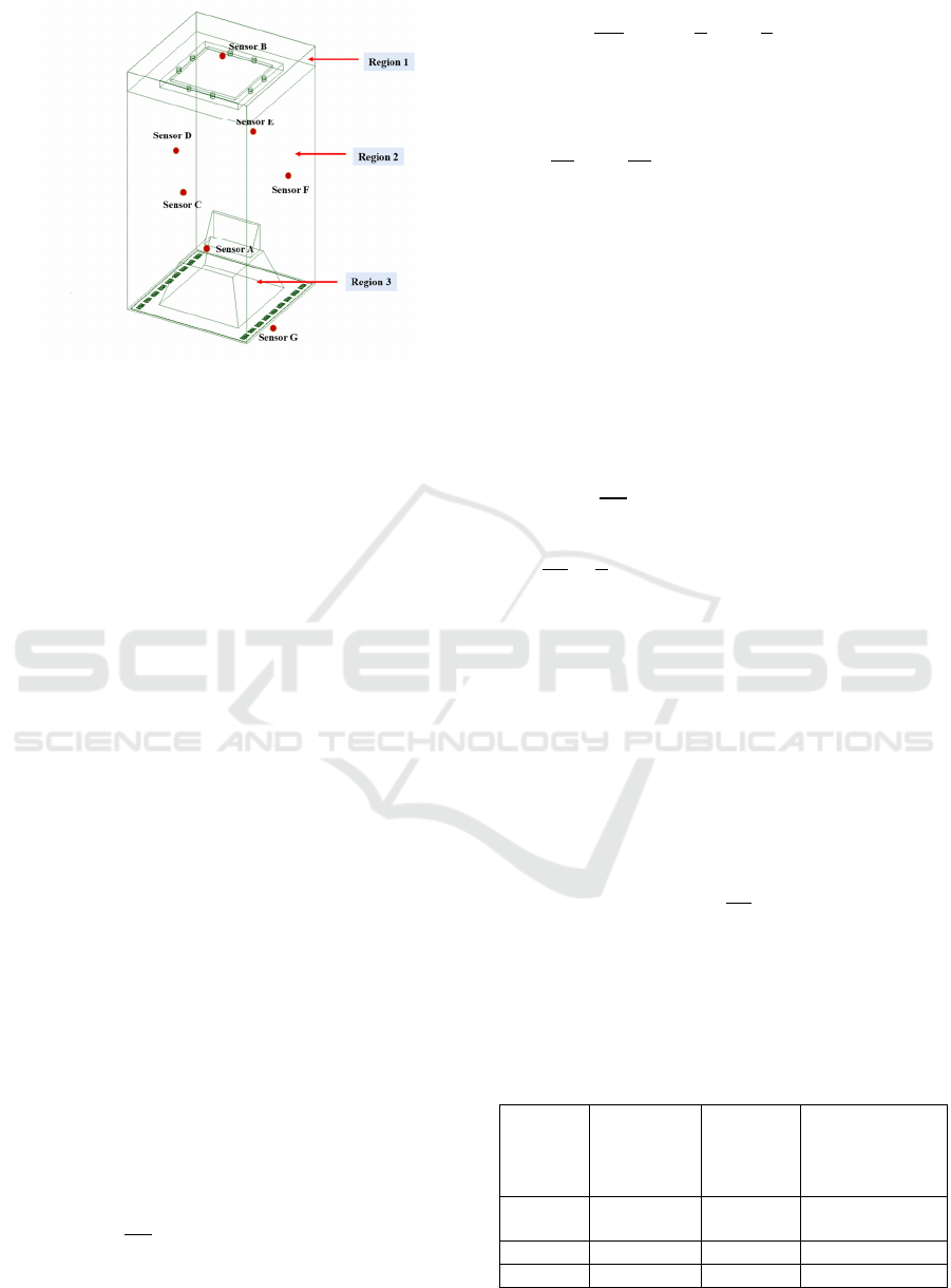
Figure 2: Geometry of the model and the sensor placement.

3 NUMERICAL METHOD

3.1 Geometry

The upper part and middle part of the showcase are

chosen as the computational domain. As shown in

Figure 2, the 3D geometry is 0.9m in length, 0.9m in

width and 1.8m in height, which are in line with actual

dimensions. Three fluid regions are created for air

flow in this computational domain as shown in Figure

2: one for the upper part of the showcase (Region 1),

one for the wooden table (Region 2) and one for the

middle part of the showcase (Region 3). There is no

direct mass transfer between the three fluid regions,

but the former two regions effect heat transfer process

in the showcase, thus they need to be taken into

account in this model, even though Region 2 is of our

most concern. It should be noted that only region 2

connects to the environment through the openings and

gaps mentioned previously. Solid regions in the

showcase model are defined to be solid materials

including aluminium, glass and wood to take into

account their effects on heat and mass transfer.

3.2 Physical Models

The coupled air flow, heat transfer and mass transfer

process in the model is calculated according to the

following physical models.

Continuity equation:

𝐷𝜌

𝐷

𝑡

+𝜌𝛻∙𝑉



⃗

=0

(1)

Momentum conservation equation, expressed by

the Navier-Stokes equation:

𝐷𝑉



⃗

𝐷𝑡

𝑓





⃗

−

𝜌

𝛻𝑝 +

𝜇

𝜌

𝛻



𝑉



⃗

)

Energy conservation equation:

𝜌

𝐷

𝐷𝑡

𝑢



𝑉



=𝜌

𝑓





⃗

∙𝑉



⃗

+∇∙𝑉



⃗

∙𝜏





+∇

(

𝜆∇𝑇

)

where 𝑡 is time, 𝜌 is air density, 𝑉



⃗

is velocity

vector, 𝑓





⃗

is volume force, 𝑝 is pressure, 𝜇 is

dynamic viscosity, 𝑢 is internal energy, 𝜏



is surface

stress components, 𝜆 is thermal conductivity, 𝑇 is

temperature.

The standard 𝑘−ε model is used to model

turbulent flow, where turbulence kinetic energy (𝑘)

and its rate of dissipation (𝜀) can be obtained from the

following equations:

𝐷𝑘

𝐷

𝑡

=𝑃



+𝐺



+𝐷



−𝜀

)

𝐷𝜀

𝐷𝑡

𝜀

𝑘

(

𝐶



𝑃



+𝐶



𝐺



−𝐶



𝜀

)

+𝐷



)

where 𝑃



is the production term of 𝑘 caused by

average speed gradient, 𝐺



is the production term of

𝑘 caused by buoyancy, 𝐷



is the diffusion term

caused by 𝑘, 𝐷



is the diffusion term caused by 𝜀, 𝐶



𝐶



and 𝐶



are model constants with values of 1.44,

1.92, and 0.09 respectively.

The one-dimension heat transfer equation is used

to describe the heat transfer process in the solid

regions with small thickness made of glass,

aluminium and wood:

𝑞=−𝜆

𝑑𝑇

𝑑𝑥

)

where q is heat flux density, λ is thermal

conductivity coefficient for certain material.

The thermal conductivity coefficients of the

materials used in this model are listed in Table 1.

Table 1: Physical parameters of the materials in the model.

Name Density(kg

)

Specific

Heat(J/kg

·K)

Thermal

conductivity

coefficients(W/

m·K)

Alumini

2719 871 202.4

Glass 2500 840 0.77

Woo

200 50 0.05

ISAIC 2022 - International Symposium on Automation, Information and Computing

312

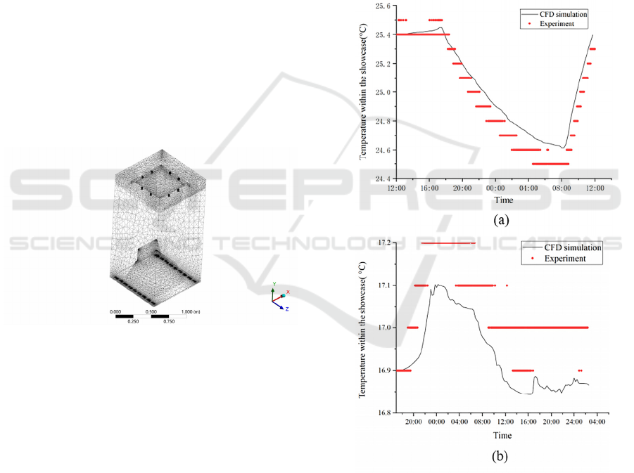
3.3 Numerical Model Settings

As shown in Figure 3, the simulation mesh in CFD is

generated based on the geometry mentioned above.

Hexahedral and tetrahedral cells are applied and the

total number of cells is 967873. The mesh is refined

at the openings and gaps in order to improve

robustness of the model. Temperature type boundary

conditions are applied to the aluminium sheet and

glass, while pressure-outlet type boundary conditions

are applied to the openings and gaps in the model.

Various environmental temperature is compiled into

UDF (User-Defined-Function) files, which are

adopted to the boundaries mentioned above. Thermal

effects of glass in the showcase are taken into account

with the shell model, in which the glass thickness,

thermal conductivity coefficient and convective heat

transfer coefficient with environment can be defined.

Thermal effects of the wooden and aluminium sheet

inside the showcase are taken into account with the

wall thickness model on interfaces between the fluid

regions. The coupled air flow, heat transfer and mass

transfer process in the model is calculated according

to the following physical models.

Figure 3: 3D Mesh for the simulation model.

4 EXPERIMENTAL VALIDATION

In order to validate the CFD model established, two

sets of experiments are performed in two typical days

in summer and winter, i.e., 14th August 2021 and

20th February 2022. The temperature data recorded

by sensors outside the showcase are adopted in the

UDFs as boundary conditions for the CFD model, so

that the air flow and temperature distribution inside

the showcase can be simulated. The measured and

simulated temperatures in summer and winter are

shown in Figure 4 as red points and black curves

respectively. The data recorded by sensor A shows

that the temperature decreases from 25.4 °C to 24.6

°C and then increases to 25.6 °C in summer, due to

the environmental temperature variation. In the

winter case, the temperature recorded by sensor A

increases from 16.9 °C to 17.2 °C and then decreases

to 16.9 °C. The measured temperature is compared

with the simulated temperature, so that prediction

accuracy of the model can be evaluated. The

comparisons show that the CFD model can predict the

temperature variation inside the showcase with

satisfactory accuracy in both cases. In the summer

case, the average and maximum deviations between

measured and simulated temperatures are 0.09 °C and

0.20 °C, respectively. In the winter case, the average

and maximum deviations between measured and

simulated temperatures are 0.06 °C and 0.10 °C,

respectively.

Figure 4: Experimental and simulated temperatures inside

the showcase: (a) The summer case; (b) The winter case.

In the validation process mentioned above, the

model gives detailed information about the

temperature and air flow distributions inside the

showcase simultaneously, and some examples are

given and discussed as follows. Two planes, i.e.,

3D Transient CFD Modelling of a Museum Showcase with Environmental Air Exchange

313

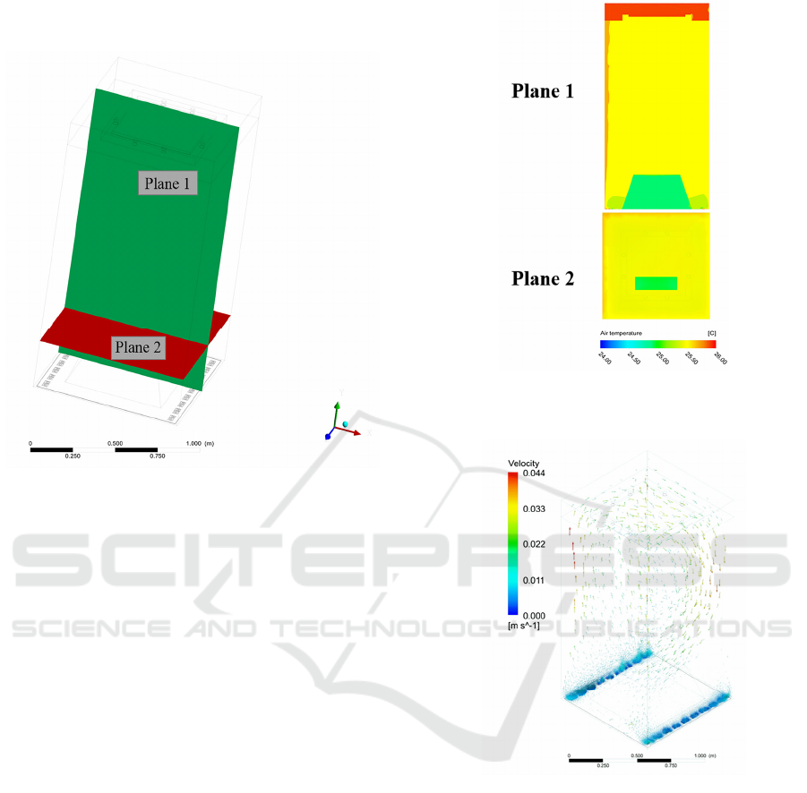
plane 1 and plane 2 in Figure 5, are created to

visualize the temperature distribution.

Figure 5: Planes for temperature visualization in the model.

Figure 6 shows the temperature distribution at a

time point in the simulation case in summer. At 12:00

of the day, the environmental temperature is higher

than the temperature inside the showcase, thus the air

inside is heated up. There are three ways of heat

transfer into the showcase in this case as follows.

Firstly, environmental air with relatively higher

temperature enters the showcase through the

openings and gaps, causing a temperature rise around

these areas. Secondly, heat transfers from the

environment into Region 1 through the aluminum

sheet enclosing this region. Due to the higher thermal

conductivity of aluminum sheet than glass, the air

temperature in Region 1 is relatively higher than that

in Region 2, which leads to the heat transfer from

Region 1 to Region 2 through the aluminum sheet

between them. Thirdly, heat transfers from the

environment into the showcase through glass and the

bottom aluminum sheet of Region 2.

The air in Region 2 has pretty uniform

distribution, which can be explained by the fact that

the convective heat transfer caused by the air flow

circulation inside this region (as shown in Figure7) is

of much higher intensity than the heat transfer into

this region caused by the three ways mentioned

above.

Figure 6: The temperature distribution at 12:00 in the

summer case.

Figure 7: The air flow distribution at 12:00 in the summer

case.

Figure 7 shows the air flow distribution in the

showcase at a time point in the simulation case in

summer. At 12:00 of the day, air in the environment

enters and mixes with the air inside the showcase

around the openings and gaps, so intense air flow and

temperature gradient form around these areas. The

temperature gradient leads to natural convection of

air, thus a convective air circulation inside the

showcase, which transfers heat simultaneously. In

this way, a coupled mass and heat transfer process is

formed.

ISAIC 2022 - International Symposium on Automation, Information and Computing

314

5 AIR EXCHANGE RATE

ANALYSIS

The CFD model established and validated

characterizes the coupled heat and mass transfer

process, so it is capable of evaluating air tightness

performance of the showcase with numerical

calculation. In order to characterize the air exchange

process between the showcase and the environment,

the carbon dioxide (CO

) tracer gas dilution

method(Xu et al., 2012) is simulated in this work. In

the CFD model, the initial CO

concentration in

Region 2 is set to be a value higher than the

environment. As air enters and exits through the gaps

and openings, the CO

in Region 2 is continuously

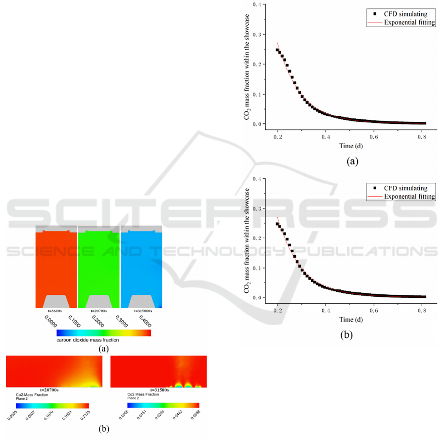
diluted. Figure 8 shows CO

concentration

distributions at different time points during the

simulation case in summer. As shown in Figure 8(a),

the CO

concentration in Region 2 decreases with

time, and is distributed uniformly at a certain time

point, which can be explained by the air circulation

inside the showcase. Figure 8(b) shows the non-

uniform CO

concentration distribution around the

openings, and the CO

concentration is lower than the

rest part of Region 2, which can be explained by the

process of air exchange with different CO

concentrations.

Figure 8: CO

concentration distributions: (a) On plane 1;

(b) Around the openings.

To characterize the CO

dilution process, the CO

concentration evolution data points are plotted with

time as black squares for the summer case and the

winter case in Figure 9. As shown in Figure 9, the

concentration decreases with time in both cases,

while an exponential relationship can be observed,

which means the rate of dilution decreases with time.

This phenomenon can be explained by the constant

and low environmental CO

concentration, which

leads to a decreasing CO

concentration difference

between the showcase and the environment, i.e., the

driving force for the CO

dilution process.

Figure 9: Simulated CO

concentration data and fitting

curves: (a) In the summer case; (b) In the winter case.

Air exchange rate is the parameter used in the one-

parameter model proposed in previous publications

to evaluate air tightness performance of a

showcase(Brimblecombe & Ramer, 1983; Calver et

al., 2005). With the data shown in Figure 9, this

parameter can be calculated and compared for the

both cases. Schematic diagram for the one-parameter

air exchange model is shown in Figure 10. Thought

of the one-parameter model is to assume that the air

exchange rate is a constant, while the air inside the

showcase is well mixed during the time period

investigated. Given the initial CO

concentration in

3D Transient CFD Modelling of a Museum Showcase with Environmental Air Exchange

315

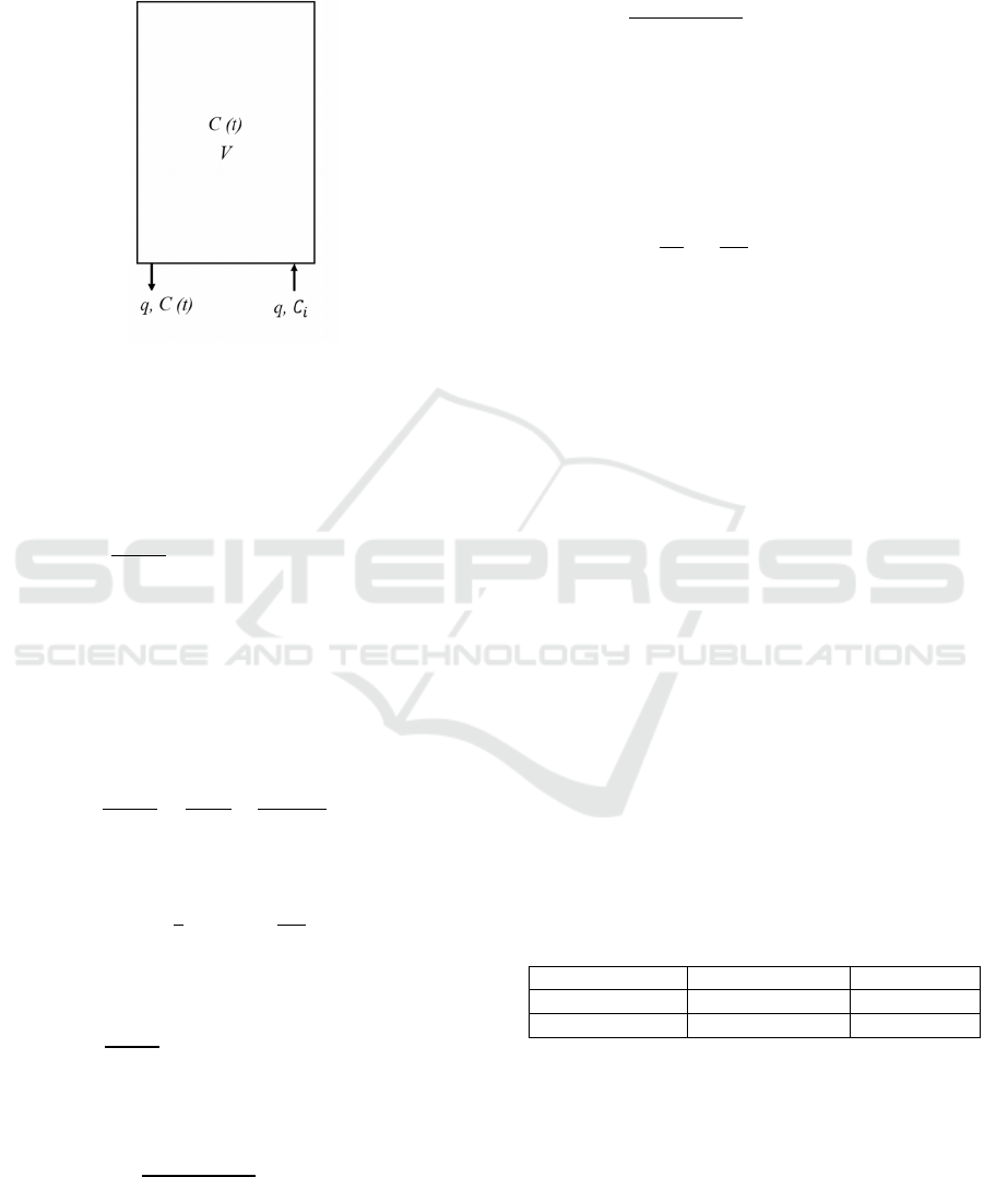
the showcase and the environmental CO

concentration, the air exchange rate of the showcase

can be calculated, and the calculation process is

illustrated as follows.

Figure 10: Schematic diagram for the one-parameter air

exchange model of museum showcases.

The CO

dilution process in the showcase can be

mathematically expressed by a differential equation

in Eq. (7), with consideration of mass balance.

𝑉

𝑑𝐶(𝑡)

𝑑𝑡

=𝑞∙𝐶



−𝑞∙𝐶(𝑡)

(7)

where 𝑉 is the volume of air inside the showcase,

𝐶(𝑡) is the average CO

concentration in the

showcase at time t, 𝐶



is the environmental CO

concentration, 𝑞 is the volumetric air flow rate of the

air exchange process.

Eq. (7) can be rewritten as:

𝑑𝐶(𝑡)

𝑑𝑡

𝑞∙𝐶



𝑉

−

𝑞∙𝐶(𝑡)

𝑉

(8)

For simplicity, let:

𝐾







and 𝐾



∙





(9)

Substituting Eq. (9) into Eq. (8) gives:

𝑑𝐶(𝑡)

𝑑𝑡

=𝐾



−𝐾



∙𝐶(𝑡)

(10)

Integrating Eq. (10) gives:



𝑑𝐶(𝑡)

𝐾



−𝐾



𝐶(𝑡)

=𝑑𝑡





()





(11)

where 𝐶



is the initial CO

concentration in the

showcase when 𝑡=0

Thus,

𝐾



−𝐾



𝐶(𝑡)

𝐾



−𝐾



𝐶



=𝑒







(12

)

Rearranging Eq. (12) leads to:

𝐾



−𝐾



𝐶(𝑡)=

(

𝐾



−𝐾



𝐶



)

𝑒







(13

)

and:

𝐶(𝑡)=

𝐾



𝐾



−

𝐾



𝐾



−𝐶



𝑒







(14

)

Substituting Eq. (9) into Eq. (14) gives the final

equation, which describes the CO

dilution process as

a function of time as Eq. (15):

(𝑡)=𝐶



−

(

𝐶



−𝐶



)

𝑒







(15

)

The exponential relationship between the CO

concentration and time agrees with the observation in

Figure 7. 𝐾



represents the air exchange rate of the

showcase with the unit of s

-1

. AER can be calculated

from 𝐾



with the unit transfer from s

-1

to d

-1

, since

AER is defined to quantify the times of air exchange

per day.

Regression calculations based on Eq. (15) are

performed with the simulated CO

concentration

evolution curves to get the parameters 𝐾



and AER,

and the AERs calculated for both cases are listed in

Tab. 2. As shown in Tab. 2, the AER in summer is

higher than that in winter, which indicates that AER

of the showcase increases with environmental

temperature. The R

values are higher than 0.99 for

both cases, which proves the model in Eq. (15) to

reflect the CFD simulation data quite well.

Table 2: Regression results for air exchange rates of the

showcase.

Condition AER/

-1

Summe

10.8 0.99857

Winte

10.0 0.99319

6 CONCLUSIONS

A 3D transient CFD model is established to

characterize the coupled air flow, heat transfer and

mass transfer phenomena in a museum showcase with

environmental air exchange in Chongqing China

ISAIC 2022 - International Symposium on Automation, Information and Computing

316

Three Gorges Museum, and the following points can

be concluded:

(1) The CFD model is successfully established and

can provide detailed information about the air

flow velocity and temperature distributions in 3D

space of the showcase at different time points

during the simulated time period.

(2) The model is validated to have high prediction

accuracy by comparing the simulated

temperature inside the showcase with

experimental data, and the average deviations are

within 0.1°C.

(3) A novel numerical CO

tracer gas dilution

method is proposed using the model established,

and the air exchange rates of the showcase can be

calculated with the method.

(4) The AER of this showcase is simulated to be 10.8

d-1 in summer and 10.0 d-1 in winter, indicating

an increase of AER with environmental

temperature.

The points above prove CFD to be a powerful tool

to model a museum showcase with environmental air

exchange, and future development of this

methodology can be expected.

ACKNOWLEDGEMENTS

This work was supported by the National Key R&D

Program of China (2020YFC1522500) and

Chongqing China Three Gorges Museum research

project (3GM2021-KTZ08).

REFERENCES

Ankersmit, B., Stappers, M. H. L., 2017. Managing Indoor

Climate Risks in Museums. Springer International

Publishing.

Balocco, C., Petrone, G., & Cammarata, G., 2014.

Numerical multi-physical approach for the assessment

of coupled heat and moisture transfer combined with

people movements in historical buildings. In Building

Simulation. Springer Berlin Heidelberg,7(3), 289-303.

Brimblecombe, P., Ramer, B., 1983. Museum display cases

and the exchange of water vapour. Studies in

Conservation, 28(4), 179–188.

Calver, A., Holbrook, A., Thickett, D., & Weintraub, S.，

2005. Simple methods to measure air exchange rates

and detect leaks in display and storage enclosures.

In ICOM Committee for Conservation: 14th Triennial

Meeting, The Hague, 12-16.

D’Agostino, D., Congedo, P. M., & Cataldo, R., 2014.

Computational fluid dynamics (CFD) modeling of

microclimate for salts crystallization control and

artworks conservation. Journal of cultural heritage,

15(4), 448-457.

Institute, G., 1994. Preventive Conservation. Care of

Collections, 83–87.

Kissel, E., 1999. The restorer: Key player in preventive

conservation. Museum International, 51(1), 33–39.

Liu, B., Yu-Ting, W. U., Chong-Fang, &M. A., 2008. CFD

Simulation of Temperature Control System for the

Museum Case of Riverside Scene at Qingming Festival.

Energy Conservation Technology, 26(6), 557-559+563.

Oetelaar, T. 2016. CFD, thermal environments, and cultural

heritage: Two case studies of Roman baths. 2016 IEEE

16th International Conference on Environment and

Electrical Engineering (EEEIC), 1–6.

Pasquarella, C., Balocco, C., Marmonti, E., Petrone, G.,

Pasquariello, G., &Albertini, R., 2013. An integrated

approach to the preventive conservation of cultural

heritage: Computational Fluid Dynamics application.

In Int. Congress Built Heritage Monitoring

Conservation Management, 18-20.

Peng, L., Nielsen, P. V., Wang, X., Sadrizadeh, S., Liu, L.,

&Li, Y., 2016. Possible user-dependent CFD

predictions of transitional flow in building ventilation.

Building and Environment, 99, 130–141.

Thomson, G., 1977. Stabilization of RH in Exhibition

Cases: Hygrometric Half-Time. Studies in

Conservation, 22, 85.

Wang, L., Xiu, G., Zhan, T., Xu, F., Wu, L., Xie, X., Zhang,

P., &Zhang, D., 2013. Impact of inlet airflow pattern on

the showcase microenvironment in museums. Sciences

of Conservation and Archaeology, 25(4), 8–13.

Xia, H., Tucker, P., Dawes, W., 2010. Level sets for CFD

in aerospace engineering. Progress in Aerospace

Sciences, 46(7), 274–283.

Xu, F., Wu, L., Xie, Y., 2012. Technology for evaluation of

showcase tightness by using tracer gases. Sciences of

Conservation and Archaeology, 24(2), 1-5.

Yi, H., Deng, C., Gong, X., Deng, X., Blatnik, M., 2021.

1D-3D Online Coupled Transient Analysis for

Powertrain-Control Integrated Thermal Management in

an Electric Vehicle. SAE International Journal of

Advances and Current Practices in Mobility, 3(2021-

01–0237), 2410–2420.

3D Transient CFD Modelling of a Museum Showcase with Environmental Air Exchange

317