A Lorentz Transition Distribution Model for High Frequency Crude

Oil Futures

Chang Liu

, Chuo Chang

and Yinglan Zhao

3,*

School of Economics and Management, University of Science and Technology Beijing, Beijing, China

PBC School of Finance, Tsinghua University, Beijing, China

School of Economics, Sichuan University, Chengdu, China

Keywords: Stochastic Volatility, Lorentz Stable Distribution, Transition Probability Distribution, Crude Oil Future.

Abstract: With the deepening of the financialization of the oil market, the importance of the oil futures market is

highlighted. The highly volatile crude oil future market inevitably has major influence on financial markets,

national economy and even national security. Therefore, modelling accurately the volatility of crude oil

futures prices has important theoretical and practical significance for investors and for preventing energy

market risks. In this paper, we study the distribution of high-frequency crude oil futures price changes.

Many empirical studies have shown that the distribution of price changes in financial market has fatter tail

than lognormal distribution. Thus, we build a model using both the transition distribution and the Lorentz

stable distribution to describe the characteristics of oil future market. Employing the Fokker-Planck

equation, we find the explicit formalism of the distribution of oil future price changes. Using empirical data

from China’s future market, we have proved the consistency of our theoretical model with the real market.

1 INTRODUCTION

In the energy structure of all countries, crude oil

constitutes one of the most crucial components. It

also plays an important part in the economic and

social development of various countries. In recent

years, the financialization of the oil market has

deepened. The oil futures market has an impact on

the price discovery of crude oil market. Therefore,

the high volatility of crude oil futures prices will

inevitably have a significant impact on financial

markets, national economy and even national

security. Therefore, modelling accurately and

estimating the volatility of crude oil futures prices

has important theoretical and practical significance

for investors, and for preventing and mitigating the

energy market risks. In this paper, we study the

distribution of high-frequency crude oil futures price

variations.

Traditionally, the solution to geometric

Brownian motion by the Black-Scholes model

(Black and Scholes, 1973; Merton, 1973) gives the

common lognormal probability distribution for

changes in financial asset prices. However, many

empirical studies have shown that the distribution of

financial assets’ price changes has fatter tail than

lognormal distribution (Bouchaud and Potters, 2003;

Wilmott, 1998).Many progress have been made

academically to improve the probability density

distribution function of financial assets. Some

scholars argue that the volatilities of financial assets

are driven by mean-reverting stochastic processes

(Engle and Patton, 2001; Blanc et al, 2014). Some

scholars believe that the volatility of financial

products should be a random variable rather than a

constant number as in Black-Scholes model (Hull

and White, 1987; Fouque et al., 2000).

Autoregressive Conditional Heteroskedasticity

models (Engle, 1982; Dumas et al., 1998) use a

function of the actual size of the error term in the

preceding time period to describe the variance of the

current error term. When the error variance is

assumed to follow the autoregressive moving

average, the model becomes a generalized

autoregressive conditional heteroskedasticity

(GARCH) model (Bollerslev, 1986; Francq and

Zakoian, 2010; Chicheportiche and Bouchaud, 2014;

Blanc et al., 2014). In financial market, GARCH

models are often applied to describe time series with

volatility clustering and time-varying volatility.

278

Liu, C., Chang, C. and Zhao, Y.

A Lorentz Transition Distribution Model for High Frequency Crude Oil Futures.

DOI: 10.5220/0011922000003612

In Proceedings of the 3rd International Symposium on Automation, Information and Computing (ISAIC 2022), pages 278-285

ISBN: 978-989-758-622-4; ISSN: 2975-9463

 2023 by SCITEPRESS – Science and Technology Publications, Lda. Under CC license (CC BY-NC-ND 4.0)

In particular, there has been extensive research

on the empirically observed power-law tails or the

scaling behaviour of financial assets (Mandelbrot,

1963; Bouchaud, 2000). Mandelbrot (1963) was the

first to notice the scaling properties of financial

assets and found that the distribution of financial

assets' price variation follows a power law. Since

then, many scholars have analyzed the power-law

distribution of financial data price tails from the

perspective of econphysics (Ballocchi et al., 1999;

Mantegna and Stanley, 1995; Ghashghaie et al.,

1996; Stanley and Plerou, 2001;Voit, 2001). Yet,

most of these studies focus on the stock and foreign

exchange markets. Many scholars have studied the

price fluctuation of crude oil market ( Wei et al.,

2010; Wen et al., 2016; Gong et al., 2017; Wei et al.,

2017; Zhang et al., 2019a; Zhang et al., 2019b; Li et

al., 2022). But there is still a lack of research on the

distribution of high-frequency crude oil futures

prices.

In this paper, we attempt to study the distribution

of high-frequency crude oil futures price changes.

We construct a two-stage distribution of a stochastic

time series for crude oil futures markets using

transition probability distribution and Lorentz stable

distribution. The Lorentz stable distribution is used

to describe the stochastic price changes of high-

frequency time series of crude oil futures. And we

use the transition distribution to model the price

transition from

𝐹



𝑡



to 𝐹



𝑡+∆𝑡



in high frequency

crude oil future market. Using Fokker-Planck

equation, we obtain the explicit expression of our

theoretical model. Using empirical data from

China’s future market, we have proved the

consistency of our theoretical model with the real

market.

The paper is organized as follows. In Section 2,

we build our theoretical model. We describe the

possible abnormal stochastic process of high-

frequency crude oil futures prices and present the

Lorentz stable distribution of high-frequency crude

oil futures prices. Then, we build the two-stage

model for the stochastic high frequency crude oil

futures market and give the explicit formalism of our

theoretical model. In Section 3, we calibrate our

theoretical model using high-frequency crude oil

future SC2209 in China’s future market. The results

show our theoretical model can describe the real

market well, with the R

=0.9849. The final section

gives the conclusion.

2 MODEL

2.1 Anomalous Geometric Brownian

Motion and Lorentz Stable

Distribution

It is generally assumed that financial asset follows

the geometric Brownian motion

𝑑𝑆=𝑆



𝜎𝑑𝐵 + 𝜇𝑑𝑡



)

In this paper, we analyse the price of future

market. We use F(t) to represent the price of the

future product at time t. Therefore, we have

𝑑𝐹=𝐹



𝜎𝑑𝐵 + 𝜇𝑑𝑡



)

Take the first order differential of time, we can

have

𝑑𝐹



𝑡



𝑑𝑡

=𝜇𝐹+𝐹𝜎𝜂



𝑡



)

where 𝜂



𝑡



represents the noise. We use a functional

probability distribution



𝑑𝑃



𝜂





to describe the

noise. Thus, the probability distribution of a

Gaussian white noise can be described as



𝑑𝑃



𝜂







𝑑𝜂



𝑒



























)

in which Ω



𝐹



depicts the width of noise

distribution.

For the Gaussian white noise, the 1-point and 2-

point correlations are characterized as

𝐸



𝜂



𝑡





=0,

𝐸



𝜂



𝑡



𝜂



𝑡′





=Ω



𝐹



𝛿



𝑡−𝑡





)

Given that for initio time 𝑡



, the value

of 𝐹



𝑡





=𝐹



, the log-return is of the form

𝑟



𝑡



=𝑙𝑛𝐹



𝑡



/𝐹0.

)

Take the first order differential of time, we can

have

𝑑𝑟



𝑡



𝑑𝑡

=𝜇−

𝜎



+𝜎𝜂



𝑡



)

We define the relative log-return 𝑧



𝑡



𝑧



𝑡



=𝑟



𝑡



−𝜇𝑡.

)

The Langevin equation of the relative log-return

𝑧



𝑡



can be written as

𝑑𝑧



𝑡



𝑑𝑡

=−

𝜎



+𝜎𝜂



𝑡



)

For the stochastic variable 𝑧



𝑡



, the probability

distribution 𝑃



𝑧,𝑡



is of the form

𝑃



𝑧,𝑡



=𝐸



𝛿𝑧



𝑡



−𝑧



(10

)

Differentiating the probability distribution

𝑃



𝑧,𝑡



and using equation (3) (Hohenberg and

Halperin, 1977), we can obtain

𝜕𝑃



𝑧,𝑡



𝜕𝑡

=𝐸



−

𝜎



+𝜎𝜂



𝑡





𝜕

𝜕𝑧



𝑡



𝛿𝑧



𝑡



−𝑧.

(11

)

The probability distribution 𝑃



𝑧,𝑡



satisfies

Fokker-Planck equation, therefore we have

A Lorentz Transition Distribution Model for High Frequency Crude Oil Futures

279

𝜕𝑃



𝑧,𝑡



𝜕𝑡

𝜕

𝜕𝑧



𝜎Ω



𝑧



𝜕𝑃



𝑧,𝑡



𝜕𝑧

+𝜎



𝑃



𝑧,𝑡





(12

)

As for the stationary solution 𝑃



𝑧



, it also

satisfies the stationary Fokker-Planck equation.

Therefore we can obtain

𝜕

𝜕𝑧

𝜎Ω



𝑧



𝜕𝑃





𝑧



𝜕𝑧

+𝜎



𝑃





𝑧



=0.

(13

)

Integrate the above equation, we can have

𝜎Ω



𝑧



𝜕𝑃





𝑧



𝜕

𝑧

+𝜎



𝑃





𝑧



=𝐶,

(14

)

where 𝐶 is an integral constant.

As 𝑧



=−∞,𝑧



=∞, the integral constant

which represents the probability current equals zero.

Therefore, this equation can be reduced as



𝑧



𝜕𝑃





𝑧



𝜕

𝑧

+𝜎𝑃





𝑧



=0.

(15

)

Solving out the stationary Fokker-Planck

equation exactly, we have

𝑃





𝑧



𝑁

exp −

𝜎



𝑧



𝑑𝑧,

(16

)

Here 𝑁 represents normalization constant.

The width of diffusion is set to be



𝑧



𝜎

𝛾



+𝑧



𝑧

(17

)

Thus, we can obtain the Lorentz distribution as

𝑃





𝑧



𝛾

𝜋

𝛾



+𝑧



(18

)

If 𝑧 is a sum of two Lorentzian random variables

𝑧



and 𝑧



, the probability density distribution of

𝑧=𝑧



+𝑧



under the assumption of independence

of 𝑧



and𝑧



𝑃





𝑧



=𝑃





𝑧





⨂𝑃





𝑧





= 𝑃





𝑧





𝑃





𝑧−𝑧









𝑑𝑧



(19

)

To calculate the probability density distribution

𝑃





𝑧



, we define the characteristic function of the

Lorentzian stochastic process

𝜙



𝑞



≡ 𝑃





𝑧





𝑒







𝑑𝑧.

(20

)

It is not difficult to get the characteristic function

of the Lorentzian stochastic process

𝜙





𝑞



=𝑒





(21

)

The convolution theorem of Fourier transform

implies that the characteristic function of the

stochastic variable

𝑧 is given by

𝜙





𝑞





𝜙





𝑞







=𝑒





(22

)

By making use of the inverse Fourier transform,

we can obtain the probability density function for

the stochastic variable 𝑧=𝑧



+𝑧



𝑃





𝑧



2𝜋

𝜙





𝑞







𝑒



𝑑𝑞

(23

)

2𝛾

𝜋

4𝛾



+𝑧



In the general case, the probability density function

for the stochastic variable 𝑧=𝑧



+𝑧



+⋯+𝑧



of the form

𝑃





𝑧



=𝑃





𝑧





⨂𝑃





𝑧





⨂⋯⨂𝑃





𝑧





= 𝑃





𝑧





𝑃





𝑧





⋯𝑃





𝑧





𝑃





𝑧−𝑧







−𝑧



−⋯−𝑧





𝑑𝑧



𝑑𝑧



⋯𝑑𝑧



(24

)

The convolution theorem of Fourier transform

guarantees that the characteristic function of the

stochastic variable 𝑧 is as

𝜙





𝑞





𝜙





𝑞







=𝑒





(25

)

Using the inverse Fourier transform, we can have the

probability density function for the stochastic

variable 𝑧=𝑧



+𝑧



+⋯+𝑧



𝑃





𝑧



2𝜋

𝜙





𝑞







𝑒



𝑑𝑞

𝑛𝛾

𝜋

𝑛



𝛾



+𝑧



(26

)

Thus, the Lorentzian distribution is stable.

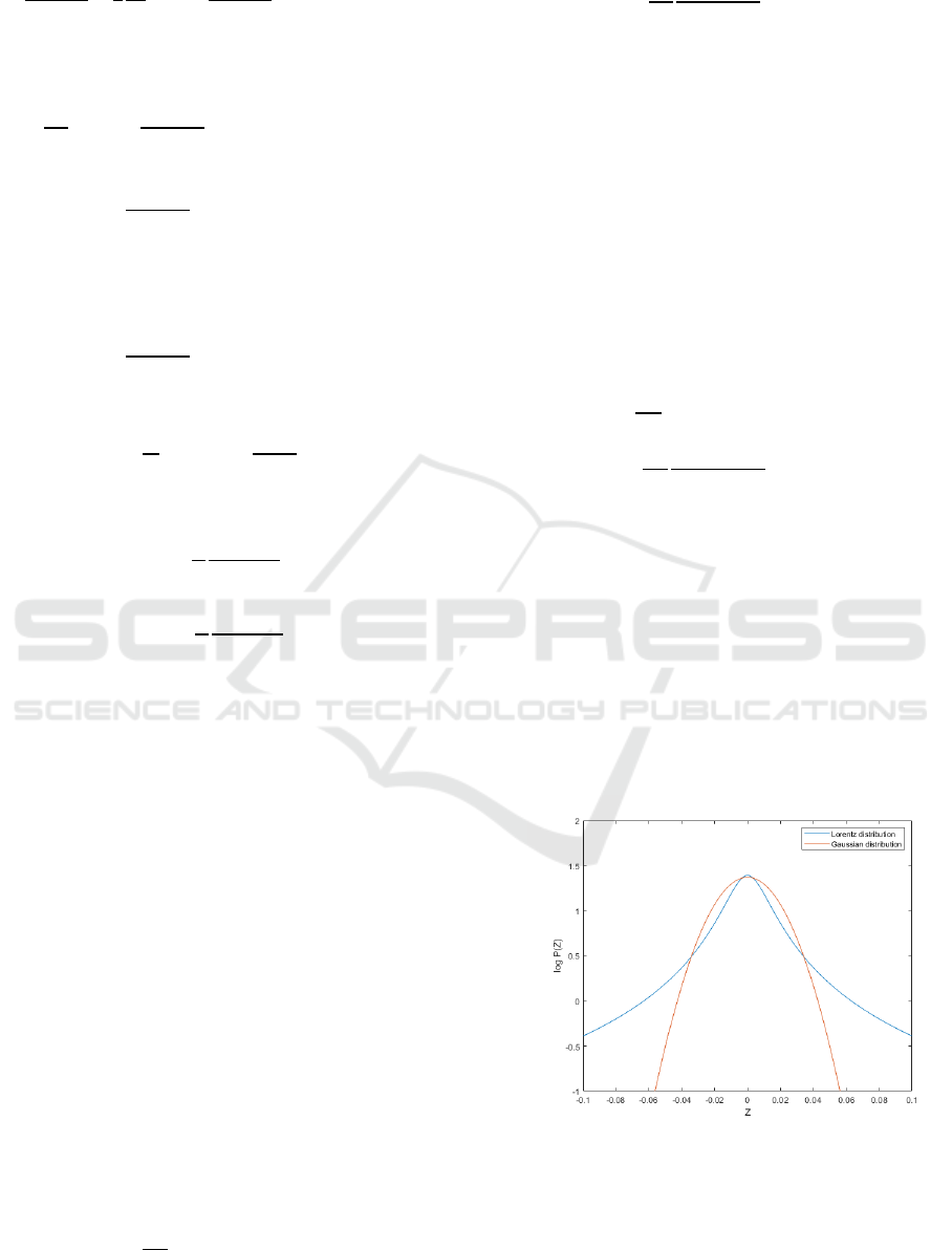
In Figure 1 and Figure 2, we exhibit the

comparison of Lorentz distribution with some other

distributions. We compare the Lorentz distribution

with the Gaussian distribution in figure 1. It can be

seen that in comparison with Gaussian distribution,

the Lorentz distribution is a better fit for the fat-tail

distribution observed in real financial market. In

figure 2, we present a comparison of truncated Lévy

flight with Lorentz distribution. When the stochastic

variable 𝑧 is relatively large, the Lorentz stable

distribution approaches 1𝑧



while the truncated

Lévy flight approaches 1𝑧

.

Figure 1: A comparison of the Gaussian distribution with

Lorentz distribution. It can be seen that in comparison

with Gaussian distribution, the Lorentz distribution is a

better fit for the fat-tail distribution observed in real

financial market.

ISAIC 2022 - International Symposium on Automation, Information and Computing

280

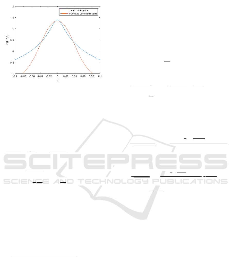
Figure 2: A comparison of Truncated Lévy flight with

Lorentz distribution. When the stochastic variable z is

relatively large, the Lorentz stable distribution approaches

1𝑧



while the truncated Levy flight approaches 1𝑧

.

2.2 The Transition Probability

Distribution

In the previous part, we have already obtained the

Fokker-Planck equation,

𝜕𝑃



𝑧,𝑡



𝜕𝑡

𝜕

𝜕𝑧



𝜎Ω



𝑧



𝜕𝑃



𝑧,𝑡



𝜕𝑧

+𝜎



𝑃



𝑧,𝑡





(27

)

We can rewrite the above Fokker-Planck equation as

𝜕𝑃



𝑧,𝑡



𝜕𝑡

=𝐿



𝑃



𝑧,𝑡



𝐿



≡

𝜕

𝜕𝑧



𝜎Ω



𝑧



𝜕

𝜕𝑧

+𝜎





(28

)

The price changes of oil future can be defined as

𝑍

∆

=𝑙𝑛𝐹



𝑡+∆𝑡



−𝑙𝑛𝐹



𝑡



(29

)

As for the probability density of 𝑧 at time 𝑡+∆𝑡

under the condition that it has the value



𝑡



, we

define the conditional probability density as

𝑃



𝑧



𝑡+∆𝑡





𝑡+∆𝑡

|

𝑧



𝑡



,𝑡



〈

𝛿



𝑧



𝑡



−𝑧



𝑡+∆𝑡





〉

(30

)

It can be deduced that for initial condition

𝑃



𝑧,𝑡



= 𝑃



𝑧



𝑡+∆𝑡





𝑡+∆𝑡

|

𝑧



𝑡



,𝑡



should also

follow the Fokker-Planck equation (28), namely

𝜕𝑃



𝑧



𝑡+∆𝑡





𝑡+∆𝑡



𝑧



𝑡



,𝑡



𝜕𝑡

=𝐿



𝑃



𝑧



𝑡+∆𝑡





𝑡+∆𝑡



𝑧



𝑡



,𝑡



(31

)

We can find one formal solution of the above

equation as

𝑃



𝑧



𝑡+∆𝑡





𝑡+∆𝑡

|

𝑧



𝑡



,𝑡



=𝑒





∆

𝛿



𝑧



𝑡+∆𝑡



−𝑧



𝑡





(32

)

Making use of iteration (Dyson, 1949), we can

obtain the following equation

𝑃



𝑧



𝑡+∆𝑡





𝑡+∆𝑡

|

𝑧



𝑡



,𝑡



=𝛿



𝑧



𝑡+∆𝑡



−𝑧



𝑡







1+Π



(33)

Π= 𝑑𝑡



∆



𝑑𝑡









⋯ 𝑑𝑡









𝐿





𝑧,𝑡





⋯𝐿





𝑧,𝑡









When the time interval ∆t is relatively small, the

solution reads

𝑃



𝑧



𝑡+∆𝑡





𝑡+∆𝑡

|

𝑧



𝑡



,𝑡



=𝛿𝑧



𝑡+∆𝑡



−𝑧



𝑡







𝐿





𝑧,𝑡



∆𝑡 + 𝑂



∆𝑡







(34

)

By using the integral presentation of the 𝛿

function, we can have

𝛿



𝑧−𝑧′



2𝜋

 𝑒

𝑖𝑢







𝑑𝑢

∞

−∞

(35

)

Thus,

𝑃



𝑧



𝑡+∆𝑡





𝑡+∆𝑡

|

𝑧



𝑡



,𝑡



1 +

𝜕



𝜕𝑧



𝑡+∆𝑡





𝜎Ω



𝑧



−

𝜕

𝜕𝑧



𝑡+∆𝑡



𝜎

𝑑Ω



𝑧



𝑑𝑧

−𝜎







2𝜋

 𝑒

𝑖𝑢







∆













𝑑𝑢

∞

−∞

(36

)

Replacing

𝑧



𝑡+∆𝑡



𝑧



𝑡



in the drift

coefficient and diffusion coefficient (Risken, 1984;

Wissel, 1979), the above equation can be rewritten

𝑃



𝑧



𝑡+∆𝑡





𝑡+∆𝑡

|

𝑧



𝑡



,𝑡



(37

)



2𝜋𝜎Ω𝑧∆𝑡

exp −

𝑍

∆

−

𝜎

𝑑Ω



𝑧



𝑑𝑧

−𝜎



∆𝑡



2𝜎Ω



𝑧



∆𝑡

Therefore, the probability density distribution of

oil future price changes

𝑍

∆

can be expressed as

𝑃



𝑍

∆







2𝜋𝜎Ω𝑧∆𝑡

exp−



𝑍

∆

−

𝜎

𝑑Ω𝑧

𝑑𝑧

−𝜎



∆𝑡





2𝜎Ω𝑧∆𝑡



𝛾

𝜋

𝛾



+𝑧



𝑑

𝑧

(38

)

Here Ω



𝑧



𝜎

𝛾

+𝑧

2𝑧

In figure 3, we compare the model we build with

Gaussian distribution and the truncated Lévy flight.

As can be seen in figure 3, in comparison with

Gaussian distribution, the Lorentz transition

distribution and truncated Lévy flight can describe

the leptokurtic feature of financial assets' price

variations better. When the price variations are

small, Lorentz transition distribution and truncated

Lévy flight perform similarly. When the price

variations are relatively large, Lorentz transition

distribution has fatter tail than truncated Lévy flight.

A Lorentz Transition Distribution Model for High Frequency Crude Oil Futures

281

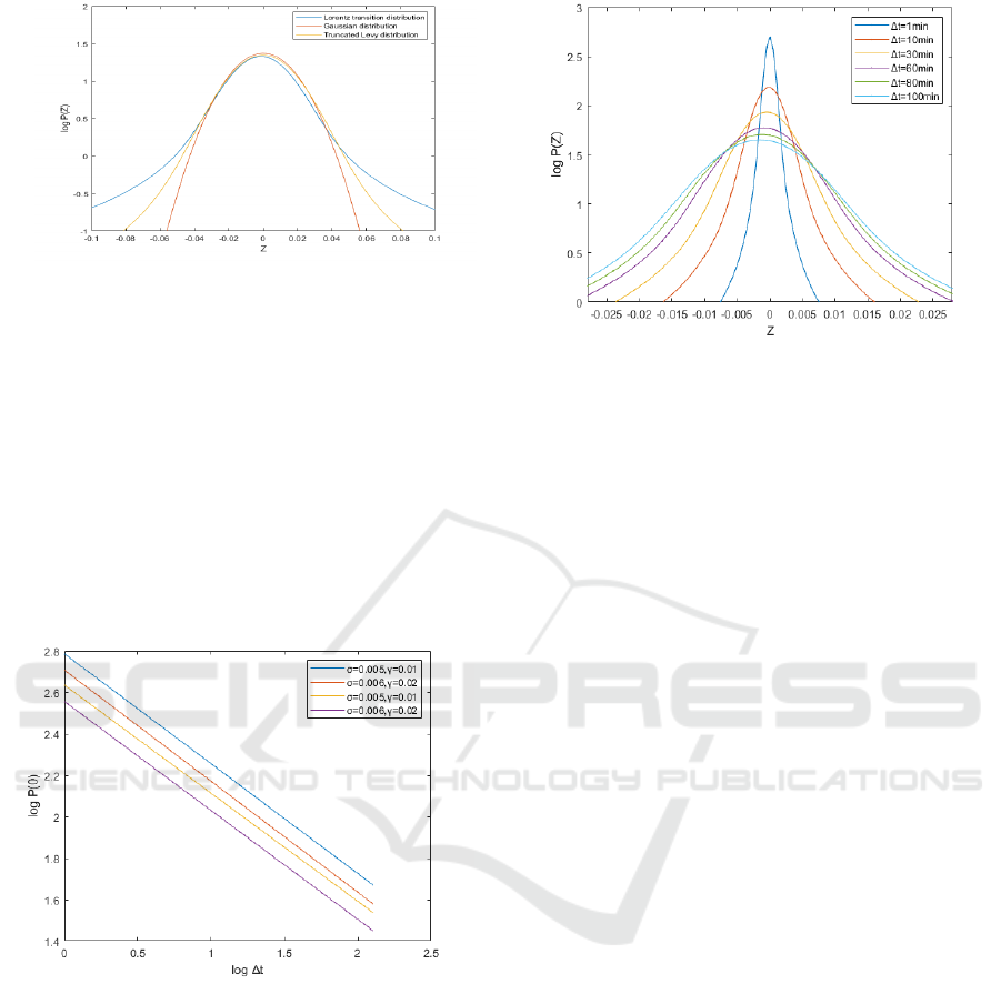
Figure 3: A comparison of distribution models. In general,

the Lorentz transition distribution and truncated Lévy

flight can describe the leptokurtic feature of financial

assets' price variations better than Gaussian distribution.

When the price variations are small, Lorentz transition

distribution and truncated Lévy flight perform similarly.

When the price variations are relatively large, Lorentz

transition distribution has fatter tail than the truncated

Lévy flight.

We calculate the correlation between the probability

of no price change and different time intervals ∆t for

different parameters

𝛾 and 𝜎 and present the result

in figure 4.

Figure 4: The correlation between the probabilities of no

price change P



∆



with the time interval ∆t.

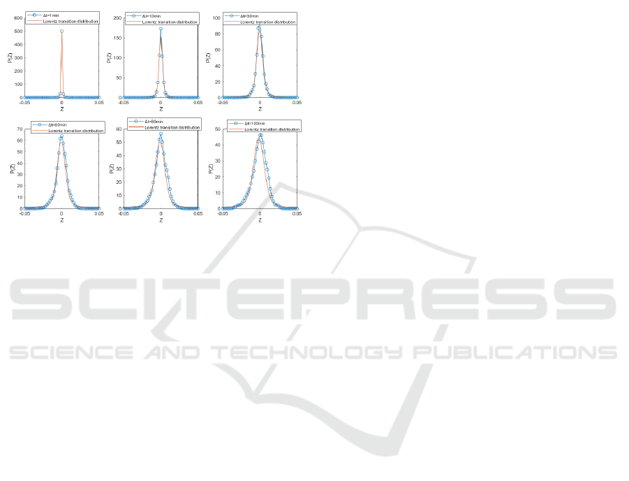
In figure 5, we plot the Lorentz transition

probability distribution of parameters

𝛾 =0.012, and

𝜎 =0.005463 for different time intervals (∆𝑡 =1, 10,

30, 60, 80 and 100 minutes) (in logarithmic form).

As can be seen in figure 5, our newly built

Lorentz transition distribution model has leptokurtic

distribution and is also mostly symmetric with finite

variance. When the time interval ∆t increases, the

Lorentz transition distribution is likely to spread.

Figure 5: The Lorentz transition probability distribution of

parameters

𝛾 =0.012, and 𝜎=0.005463 for different

time intervals

(∆𝑡 =1, 10, 30, 60, 80 and 100 minutes).

Lorentz transition distribution model has leptokurtic

distribution and is also mostly symmetric with finite

variance. When the time interval ∆t increases, the Lorentz

transition distribution is likely to spread.

3 CALIBRATION OF THE

MODEL IN CRUDE OIL

FUTURE MARKET

Now, we try to analyse statistically the features of

the high frequency crude oil future in China's future

market by using the new distribution model that we

developed at last sections. We obtain the 1-minute

high frequency data of crude oil future SC2209 from

the Wind database. Our data period ranges from

May 11, 2022, to August 4, 2022. We denote the

price of crude oil future SC2209 as 𝐹



𝑡



, and the

successive variation of the crude oil future price is

denoted as 𝑍

∆

The price changes of the crude oil future SC2209

is measured as follows:

𝑍

∆

=𝑙𝑛𝐹



𝑡+∆𝑡



−𝑙𝑛𝐹



𝑡



(39

)

We calculate the probability distribution 𝑃



𝑍

∆



of crude oil future price variations for different time

values ( ∆𝑡 =1, 10, 30, 60, 80 and 100 minutes).

Figure 6 and 7 are semilogarithmic plots of

𝑃



𝑍

∆



different time interval ∆𝑡. As can be seen in figure 6

and figure 7, the distribution of high frequency crude

oil futures have fatter tail than log-normal

distribution. The crude oil future price variations

cannot be depicted well by a random walk. The

distributions are leptokurtic and tend to spread as the

time interval ∆𝑡 increases.

ISAIC 2022 - International Symposium on Automation, Information and Computing

282

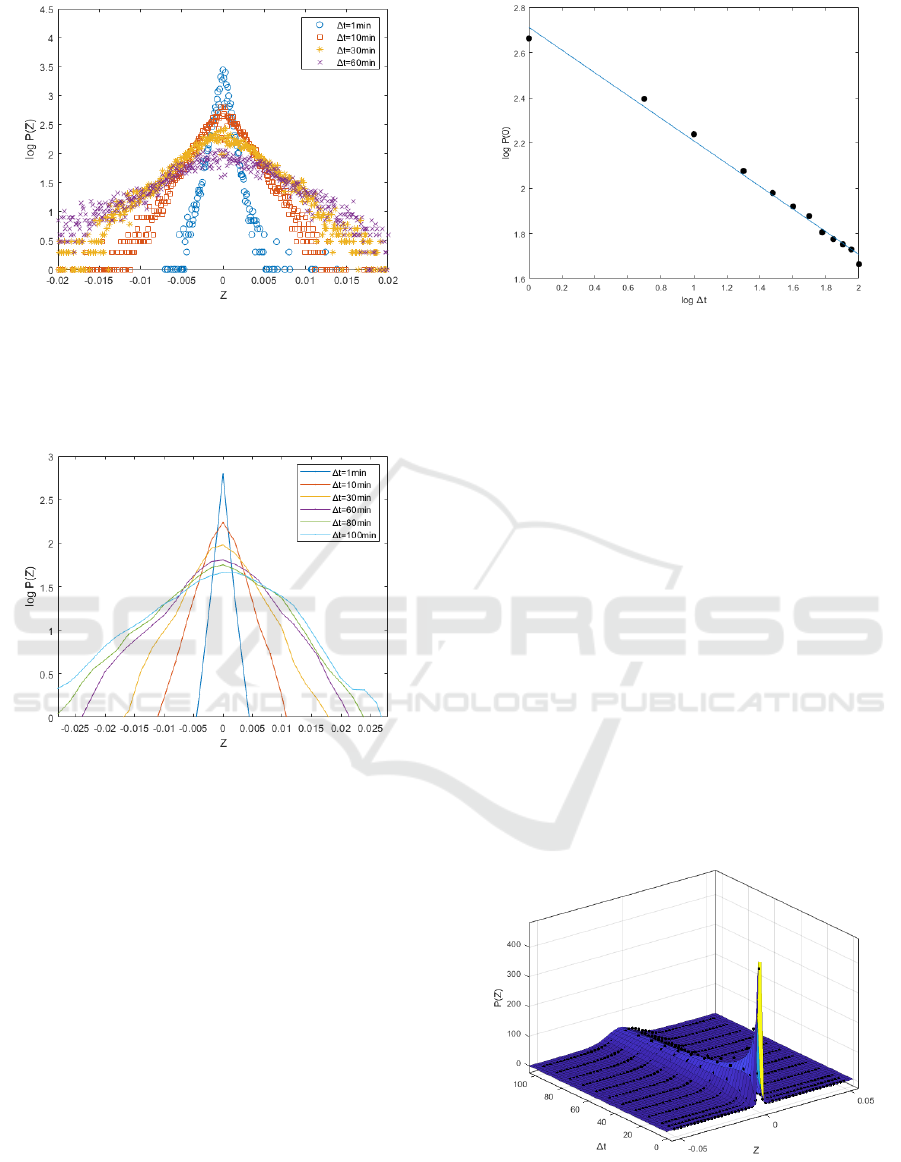
Figure 6: Probability density distributions 𝑃



𝑍

∆



of crude

oil future price variation measured at different time

intervals (∆𝑡) 1, 10, 30 and 60 minutes for high-frequency

data in China's future market during the period from May

11, 2022, to August 4, 2022.

Figure 7: Probability density distributions 𝑃



𝑍

∆



of crude

oil future price variation at different time intervals (∆t) 1,

10, 30, 60, 80 and 100 minutes for high-frequency data in

China's future market during the period from May 11,

2022, to August 4, 2022.

In figure 8, we exhibit the correlation between

the probability of no price change

𝑃



𝑍

∆



and the

time interval ∆𝑡. The regression of log𝑃



𝑍

∆𝑡



log∆𝑡 gives a coefficient of -0.5019 with 95%

confidence bounds.

Figure 8: The correlation between the probability of no

price change 𝑃



𝑍

∆



for the crude oil future SC2209

and different time intervals ∆t. The slope of best-fit

straight line is -0.5019.

Now, it’s time for us to give a best-fit of the high

frequency crude oil future SC2209 by using the

Lorentz transition probability distribution. We use

the Matlab fitting toolbox to find the best-fit

parameters for our theoretical model. The best-fit of

the Lorentz transition probability distribution has the

parameters

𝛾 = 0.012, and 𝜎=0.005463 with the high

frequency crude oil future SC2209 during the period

from May 11, 2022, to August 4, 2022.The R

0.9849.The fitting results are shown in figure 9. The

high R

of the fitting result indicate that our

theoretical model can describe the characteristics of

crude oil future distribution well. As accurate

modelling and predicting the volatility of crude oil

futures prices has important theoretical and practical

significance for investors, and for preventing and

mitigating the energy market risks. The Lorentz

transition model with its accuracy can be applied

empirically.

Figure 9: The best-fit of Lorentz transition probability

distribution of parameters γ = 0.012, and σ=0.005463 with

the crude oil future SC2209 time series during the period

from May 11, 2022, to August 4, 2022.The R

is 0.9849.

A Lorentz Transition Distribution Model for High Frequency Crude Oil Futures

283

To show the calibration results clearer, in figure

10, we exhibit the best-fit of Lorentz transition

distribution with the high frequency crude oil future

SC2209 during the period from May 11, 2022, to

August 4, 2022 with different time interval ∆t=1, 10,

30, 60, 80, 100 minutes, respectively. As can be seen

in figure 10, the Lorentz transition probability

distribution describes well the price variation

distribution of crude oil future SC2209.

Figure 10: The best-fit of the probability density

distributions P



∆



of price variation for the crude oil

future SC2209 with time interval ∆t=1, 10, 30, 60, 80, 100

minutes with γ = 0.012, and σ=0.005463.

4 CONCLUDING REMARKS

With the deepening of the financialization of the oil

market, the importance of the oil futures market is

highlighted. The high volatility of crude oil futures

prices inevitably has a major influence on global

financial markets and the healthy development of

world economy. Therefore, modelling accurately

and estimating the volatility of crude oil futures

prices has important theoretical and practical

significance for investors and for preventing energy

market risks. In this paper, we study the distribution

of high- frequency crude oil futures price changes.

Many empirical studies have shown that the

distribution of financial assets’ price changes has

fatter tail than lognormal distribution. Various

efforts have been made to improve the modelling of

financial assets’ price variations. In particular, many

scholars have paid special attention to the power-law

tail and scaling property of the price variation

distributions. In this paper, we try to model the

leptokurtic distribution of high frequency crude oil

futures using a combination of transition probability

distribution and Lorentz stable distribution. The

newly built model has fatter tail than log-normal

distributions. Using high frequency data of crude oil

future in China’s future market, we calibrate our

theoretical model and have proved the consistency

of our theoretical model with the real market.

ACKNOWLEDGEMENTS

We appreciate Prof. Xiang-Bin Yan for useful

discussions and encouragements. This work was

supported by the China Postdoctoral Science

Foundation (Grant No.2021M700398).

REFERENCES

Ballocchi, G., Dacorogna, M. M., Gencay, R., and

Piccinato, B. (1999). Intraday statistical properties of

Eurofutures. Derivatives Quarterly, 6: 28-44.

Black, F. and Scholes, M.,(1973). The pricing of options

and corporate liabilities. Journal of Political Economy,

81: 637-659.

Blanc, P. Chicheportiche, R., and Bouchaud, J. P. (2014).

The fine structure of volatility feedback II: Overnight

and intra-day effects. Physica A: Statistical Mechanics

and its Applications, 402: 58-75.

Bollerslev,T.(1986). Generalized Autoregressive

Conditional Heteroskedasticity. Journal of

Econometrics, 31(3): 307-327.

Bouchaud J. P. and Potters, M. (2003). Theory of

Financial Risk and Derivative Pricing: from

Statistical Physics to Risk Management . Cambridge

University Press, Cambridge, 2nd edition.

Bouchaud, J. P. (2000). Power-laws in economy and

finance: some ideas from physics,

https://arxiv.org/pdf/cond-mat/0008103v1.

Chicheportiche R. and Bouchaud, J. P. (2014). The fine-

structure of volatility feedback I: Multi-scale self-

reflexivity. Physica A: Statistical Mechanics and its

Applications, 410: 174-195.

Dumas, B. Fleming, J., and Whaley, R. (1998). Implied

volatility functions: empirical tests. Journal of

Finance, 53(6) : 2059-2106.

Dyson, F. J. (1949). The radiation theories of Tomonaga,

Schwinger, and Feynman. Phys. Rev. 75: 486-502.

Engle R. F. and Patton, A.J. (2001). What good is a

Volatility Model? Quantitative Finance, (2) :237-245.

Engle, R. F. (1982). Autoregressive conditional

heteroscedasticity with estimates of the variance of

United Kingdom Inflation. Econometrica, 50(4): 987-

1007.

Fouque, J. P. Papanicolaou G., and Sircar, R.(2000).

Mean-Reverting Stochastic Volatility. International

Journal of Theoretical and Applied Finance, 3(1):

101-142.

ISAIC 2022 - International Symposium on Automation, Information and Computing

284

Francq C. and Zakoian, J. (2010). GARCH Models, in

Structure, statistical inference and financial

applications. Wiley, UK.

Ghashghaie, S., Breymann, W., Peinke, J., Talkner, P., and

Dodge, Y. (1996). Turbulent cascades in foreign

exchange markets. Nature, 381: 767-770.

Gong,X., Wen, F., Xia, X.H., Huang, J., and Pan, B.

(2017). Investigating the risk-return trade-off for crude

oil futures using high-frequency data. Applied Energy,

196: 152-161.

Hohenberg P. C. and Halperin, B. I. (1977). Theory of

dynamic critical phenomena. Reviews of Modem

Physics, 49: 435-478.

Hull J. and White, A. (1987). The pricing of options with

stochastic volatilities. Journal of Finance, 42: 281-

300.

Li, X. Wei, Y. Chen, X. Ma, F. Liang, C. and Chen, W.

(2022). Which uncertainty is powerful to forecast

crude oil market volatility? New evidence. Journal of

International Money and Finance, 27(4): 4279-4297.

Mandelbrot, B. B. (1963). The Variation of Certain

Speculative Prices. Journal of Business, 36: 394-419.

Mantegna R. N. and Stanley, H. E. (1995). Scaling

Behaviour in the Dynamics of an Economic Index.

Nature, 376: 46-49.

Merton, R. (1973). Theory of rational option pricing. Bell

Journal of Economics, 4:141-183.

Risken, H. (1984). The Fokker-Planck Equation. Springer-

Verlag, Berlin.

Stanley H. E. and Plerou, V. (2001). Scaling and

universality in economics: empirical results and

theoretical interpretation. Quantitative Finance, 1:563-

567.

Voit, J. (2001).The Statistical Mechanics of Financial

Markets. Springer, Berlin.

Wei, Y., Liu, J., Lai, X., and Hu, Y. (2017). Which

determinant is the most informative in forecasting

crude oil market volatility: fundamental, speculation,

or uncertainty? Energy Economics, 68:141-150.

Wei, Y., Wang, Y., and Huang D. (2010). Forecasting

crude oil market volatility: further evidence using

GARCH-class models. Energy Economics, 32:1477-

1484.

Wen, F., Gong, X., and Cai, S. (2016). Forecasting the

volatility of crude oil futures using HAR-type models

with structural breaks. Energy Economics, 59:400-

413.

Wilmott, P.(1998). Derivatives. John Wiley & Sons, New

York.

Wissel, C. (1979). Manifolds of Equivalent Path Integral

Solutions of the Fokker-Planck Equation. Z. Physik B,

35:185-191.

Zhang, Y. Ma, F. and Wang, Y. (2019a). Forecasting

crude oil prices with a large set of predictors: can

LASSO select powerful predictors? Journal of

Empirical Finance, 54:97-117.

Zhang, Y., Ma, F., and Wei, Y. (2019b). Out-of-sample

prediction of the oil futures market volatility: a

comparison of new and traditional combination

approaches. Energy Economics, 81:1109-1120.

A Lorentz Transition Distribution Model for High Frequency Crude Oil Futures

285