Research on Farmland Extraction from Remote Sensing Images
Based on Decision Tree
Liang Wu
1,*
and LanPing Xiao
2,†
1
School of Information and Media, Hubei Land Resources Vocational College Wuhan, Hubei, 430090, China
2
School of Computer Science, China University of Geosciences, Wuhan, Hubei, 430074, China
Keywords: Decision Tree, Random Forest, Remote Sensing Image, Cropland Information Extraction.
Abstract: In recent years, along with the rapid development of science and technology and the rapid increase of China's
population, urbanization has become more and more serious, and the decrease of arable land will directly lead
to food crisis and thus social problems, therefore, the statistical monitoring of arable land area is especially
important. In this paper, we propose a random forest-based construction of multiple decision tree model to
segment and extract remote sensing image plots for research. In this paper, a graph theory-based segmentation
method is used for image segmentation, and the Canny edge operator is introduced to extract edge information,
which is used to suppress the over-segmentation phenomenon generated by it. Next, it is optimized using a
Bagging-based random forest expansion algorithm. We conducted experiments on the hyperspectral remote
sensing image number dataset captured by the Resource 3 (ZY-3) satellite provided by MathorCup, and finally
obtained an accuracy of 88.09%.
1 INTRODUCTION
In recent years, along with the rapid development of
science and technology and the rapid increase of our
population, urbanization has become more and more
serious, and the decrease of arable land can directly
lead to food crisis and thus social problems.
Therefore, we investigate this problem from the
perspective of image classification.
The first proposed image segmentation algorithms
were threshold-based and edge-region-based
segmentation methods, and Felzenszwalb and
Huttenlocher (Felzenszwalb & Huttenlocher, 2004)
proposed an efficient graph-based image
segmentation theory in 2004 to achieve the retention
of detailed features in regions with a low degree of
variability while ignoring height variation and
regional detail features. In 2018, Ratna Saha,Mariusz
Bajger and Gobert Lee
(R. et al., 2018) proposed a
study using graph based segmentation approach to
segment nucleus from cytology images. In the same
year, Cahuina, Edward Cayllahua and his team
(Cahuina et al., 2018) propose a series of algorithms
to compute the result of the hierarchical graph-based
image segmentation method. In 2019, Cahuina,
Edward Cayllahua and his team (Cahuina et al., 2019)
is devoted to providing a series of algorithms to
compute the result of this hierarchical graph-based
image segmentation method efficiently. In the same
year, Shirly, S and Ramesh, K (Shirly & Ramesh,
2019) provided an insight about different 2-
Dimensional and 3-Dimensional MRI image
segmentation techniques and summarized the
benefits and limitations of various segmentation
techniques.
This paper describes the construction method of
the model, firstly, after pre-processing the image by
filtering and selecting the features, it introduces the
optimization of image segmentation by introducing
the Canny edge operator, then it introduces the
random forest to upgrade the decision tree, and finally
the experimental results are obtained after removing
the image noise, and the performance of the model on
the dataset is analyzed.
Wu, L. and Xiao, L.
Research on Farmland Extraction from Remote Sensing Images Based on Decision Tree.
DOI: 10.5220/0011918000003612
In Proceedings of the 3rd International Symposium on Automation, Information and Computing (ISAIC 2022), pages 209-215
ISBN: 978-989-758-622-4; ISSN: 2975-9463
Copyright
c
 2023 by SCITEPRESS – Science and Technology Publications, Lda. Under CC license (CC BY-NC-ND 4.0)
209

2 RELATED WORK
2.1 Image Segmentation
2.1.1 Edge Detection
The edge detection mainly consists of five steps, such
as grayscale processing, filtering fuzzy, gradient
calculation, etc. The specific algorithms are as
follows.
(1) Grayscale processing. A color image is
converted into a grayscale image by making the R, G,
and B components of the color equal.
The grayscale processing in this paper is
performed using the weighted average method with
the formula shown in equation (1).
𝐺𝑟𝑎𝑦
(
𝑖,𝑗
)
= 0.299 ∗ 𝑅
(
𝑖,𝑗
)
+ 0.578 ∗𝐺
(
𝑖,𝑗
)
+
0.114 ∗ 𝐵
(
𝑖,𝑗
)(
1
)
(2) Processing by bilateral filtering method.
(3) Calculating gradient value and direction.
Image gradient is the partial derivative of the pixel
point currently located for the X and Y axes, and the
gradient is the rate of change of the pixel gray value
in the image processing field. Defined as the image
gray value, assigned to the X-direction gradient,
assigned to the Y-direction gradient, assigned to the
point, the gradient direction (angle), as shown in
equation (2).
𝑃(𝑖,𝑗)= (𝑓(𝑖− 1,𝑗) − 𝑓(𝑖,𝑗) + 𝑓(𝑖 +1,𝑗+ 1)
− 𝑓(𝑖,𝑗+1))/2
𝑄(𝑖,𝑗)= (𝑓(𝑖,𝑗) −𝑓(𝑖,𝑗 +1)+𝑓(𝑖 + 1,𝑗)− 𝑓(𝑖
+1,𝑗+1))/2
𝑀(𝑖,𝑗) =

𝑃(𝑖,𝑗)

+𝑄(𝑖,𝑗)

𝜃
(
𝑖,𝑗
)
=
𝑎𝑟𝑐𝑡𝑎𝑛(𝑄
(
𝑖,𝑗
)
𝑃
(
𝑖,𝑗
)
(
2
)
(4) Non-maximum suppression. The idea of non-
maximal suppression is to search for the local
maximum gradient and retain it, and sieve out all
other non-maximal values. The specific steps are as
follows.
1. Compare the gradient intensity of the current
point with the gradient intensity of the points in the
positive and negative gradient directions.
2. If the gradient intensity of the current point is
the maximum compared to other points in its same
direction, then keep it. Otherwise, it is suppressed, i.e.
set to 0.
(5) Edge connection. While most of the other
conventional algorithms filter out small gradients
caused by noise or color changes while maintaining
larger gradients by using a threshold, the Canny
algorithm uses a double threshold, i.e., a low TL
threshold and a high TH threshold to separate edge
pixels. According to TL and TH, a point less than TL
is set with a 0 marker when connecting the edges of
an image; points greater than T H are assigned a value
of 1. The 8-connected region is used to define the
point between TL and TH, and when a TH pixel point
exists in the 8-connected region, it should be
designated as a polar point.
2.1.2 Figure Cut Chunking
In the original scheme, it judges whether two regions
should be merged based on the inter-region spacing
and intra-region spacing. In this paper, based on the
extracted edge information, we set the edge weight of
adjacent nodes at the edge to infinity to suppress the
under-segmentation and over-segmentation
phenomena.
Using the satellite image of RBG and the binary
image of edge detection as input, the image content is
blocked in the following steps.
Let each pixel point of the RGB satellite image be
a separate node, and each pixel point is connected
with other pixel points in its four-neighborhood range
to form 𝐺=
(
𝑉,𝐸
)
, where the edge weights of the
edges (𝑣

,𝑣

) are their Euclidean distances in the
RGB space, as shown in equation (3).
𝑤
,
=

(𝑅

−𝑅

)

+(𝐺

−𝐺

)

+(𝐵

−𝐵

)

(
3
)
Define as the set of edges obtained by edge
extraction, introducing edge information to restrict
the edge weights when 𝑣

,𝑣

∉𝑒𝑑𝑔𝑒 as shown in
equation (4), when 𝑣

|𝑣

∈𝑒𝑑𝑔𝑒, taking ∞ as shown
in.
𝑤


,

=

𝑅

−𝑅



+𝐺

−𝐺



+𝐵

−𝐵



(
4
)
Define the inter-region spacing as shown in
equation (5).
𝐷𝑖𝑓
(
𝐶

,𝐶

)
=𝑚𝑖𝑛


∈

,

∈

,



,


∈
𝜔


,

(
5
)
The intra-definition interval spacing is shown in
equation (6).
𝑀𝑖𝑛𝑡(𝐶) = 𝑚𝑎𝑥
∈
(
,
)
𝑤
(
𝑒
)
+
𝐾
|
𝐶
|
(6)
where MST denotes the minimum spanning tree of
region C, which is defined here as the maximum
connected edge length in the region, k is a constant,
and |C| denotes the number of nodes in the region.
The final judgment basis for region merging is
obtained by comparing the size relationship between
𝐷𝑖𝑓(𝐶

,𝐶

)and 𝑚𝑖𝑛(𝑀 𝑖𝑛𝑡(𝐶

),𝑀 𝑖𝑛𝑡(𝐶

)).
Since the edge detection picture is combined in
the construction of the graph structure, for the edge
neighbouring points detected in the Canny edge
detection in the graph the edge weight is infinite, that
ISAIC 2022 - International Symposium on Automation, Information and Computing
210

is, the edge information in the edge picture is used as
one of the bases for the chunking, so the process of
the graph cut chunking can better segment different
regions and reduce the phenomenon of incomplete
and inappropriate segmentation.
After chunking, the satellite map of farmland can
be more complete to divide each object in the image
as a whole, after chunking, a piece of farmland in the
image is divided out individually, and the subsequent
processing takes each area as the processing object.
This helps to retain the image characteristics and
integrity of the farmland block as a whole. And for
different farmland blocks, their colour and other
characteristics may be different, and by segmenting
each object in the image, it is possible to process
different farmland types, forests, houses and other
information separately.
2.2 Decision Tree
The decision tree is a tree structure that uses layer by
layer inference to achieve classification, and its
internal nodes are divided into three categories: one
is the root node, which contains the full set of
samples; the second is the internal node, which is
used to perform feature attribute testing and decide
the direction of the next decision; the third is the leaf
node, each leaf node contains a definite classification
result, and when the attribute test goes to the leaf node
means the end of the decision. The main steps of the
algorithm are as follows.
(1) Collecting samples.
(2) Select features and construct nodes. According
to the importance of features to construct sub-nodes,
the more important features are closer to the root
node, the more representative genes are selected as
features in this problem, the closer genes are to the
root node, the importance of genes can be judged by
calculating information entropy and Gini coefficient,
the formula is shown in equation (7).
𝐻
(
𝑋
)
=−𝑝
(
𝑥
)
𝑙𝑜𝑔𝑝
(
𝑥
)
∈
(
7
)
Where p(x) represents the probability that a value
x can be taken. Assuming that there is a sample set D,
the discrete attribute a has N possible value
{𝑎

,𝑎

,...𝑎

}, using the partition of the sample set a,
N branching node is created. The i branch node
contains all the samples D in the attribute a with
entropy values
i
a
, which is denoted as 𝐷

.
The formula for calculating the Gini coefficient is
shown in equation (8).
𝐺𝑎𝑖𝑛
(
𝐷
)
=𝑝

(
1−𝑝

)
=1−𝑝






(
8
)
The Gini coefficient reflects the probability that
two samples are randomly selected from the dataset
D with different labels. The smaller the Gini
coefficient, the higher the purity of the dataset D.
The Gini coefficient of set D under attribute a is
defined as shown in equation (9).
𝐺𝑎𝑖𝑛
(
𝐷,𝑎
)
=
𝐷


|
𝐷
|
𝐺𝑖𝑛𝑖
(
𝐷

)


(
9
)
Some value of attribute a divides D into two parts
𝐷

and 𝐷

, at which point the Gini coefficient is
shown in equation (10).
𝐺𝑎𝑖𝑛
(
𝐷,𝑎
)
=
|
𝐷

|
|
𝐷
|
𝐷𝑖𝑛𝑖
(
𝐷

)
+
|
𝐷

|
|
𝐷
|
𝐷𝑖𝑛𝑖
(
𝐷

)(
10
)
(3) Split nodes. Divide the dataset according to the
way the features are split, i.e., differentiate according
to the conditions.
3 THE IMPROVEMENT
3.1 Random Forest
A random forest is a classifier consisting of multiple
unrelated decision trees. When performing a
classification task, each time a new sample is input,
each decision tree in the forest is allowed to classify
and get multiple identical or different results, using
voting to get the final forest classification result. Its
integrated method implementation based on Bagging
makes the accuracy of decision trees rise another big
step. The basic steps of its algorithm are as follows.
(1) Divide the training set into n subsets, using m
to represent the total number of features.
(2) Input the number of features m, which is used
to determine the decision outcome of a node on the
decision tree; where m should be much smaller than
n.
(3) Create a training set and predict non-negative
example errors by sampling n times from the n
subsets in a way that has put-back sampling to
evaluate the error.
(4) For each node arbitrarily choose m features
and calculate its optimal split based on these m
features.
(5) Make each tree grow fully instead of pruning
branches.
(6) Classify the new data using a random forest
classifier composed of the generated multiple
decision trees, and decide the classification result
according to how many votes the tree classifier has.
Research on Farmland Extraction from Remote Sensing Images Based on Decision Tree
211

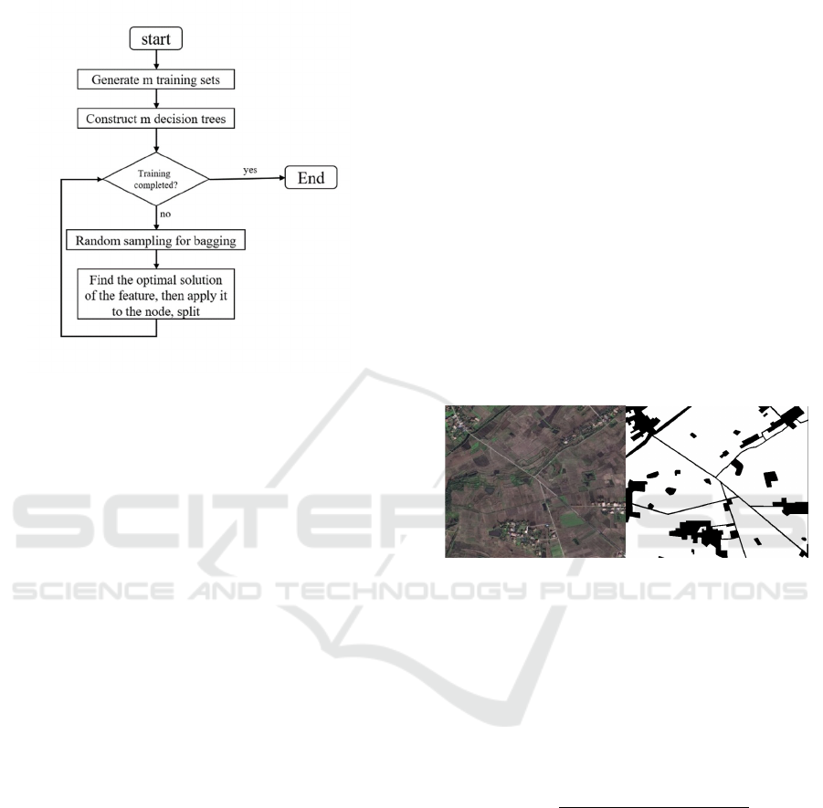
The flowchart of the algorithm is shown in Figure
1.
Figure 1: Random forest model flowchart
3.2 Output Image Denoising
Due to the introduction of the Canny edge operator,
less edge information is retained in the resultant
image. The image is processed using the image
erosion expansion operation and the open-close
operation, which can effectively remove the
redundant edge information while retaining the
original shape of the image, with good suppression of
edge noise and improved accuracy.
Erosion operation takes the smallest value in the
rectangular neighborhood of each position as the
output gray value of that position and reduces the gray
value, so that the area of bright areas in the image will
become smaller and the area of dark areas will
increase.
In contrast to erosion, the expansion operation
expands the brighter part of the image by finding the
local maximum, so that this part has a larger area in
the effect image compared with the original image,
i.e. the brighter objects in the image will be larger in
size and the darker objects will be smaller in size.
The open operation eliminates the small brighter
areas in the image by first eroding and then
expanding, while the closed operation removes the
small black voids in the image by first expanding and
then eroding. Both algorithms do not change the area
of other objects.
4 EXPERIMENTS PROCESS AND
RESLUT ANALYSIS
4.1 Data Sets
The dataset used in this experiment is from the
MathorCup Collegiate Mathematical Modeling
Challenge. The images were obtained from remote
sensing image data acquired by the Resource 3
satellite, China's first autonomous civilian high-
resolution stereo mapping satellite, with a spatial
resolution of 2 m and a spectrum in the visible band
(red, green, and blue). This dataset contains a total of
ten hyperspectral remote sensing images, and
includes labels (labels) labeled by professionals for
cultivated land. In this experiment, we divide the
dataset according to the ratio of 4:1, with the first 80%
as the training set and 20% as the validation set. An
example of the dataset is shown in Figure 2, with the
tif image visualized on the left, the label map on the
right, and the cultivated land in black.
Figure 2: Example data set
4.2 Evaluation Indicators
For a single figure, the evaluation method is to use the
model to predict the labeled figure and compare it
with the standard labeled figure, and calculate the
accuracy based on the number of pixels and the
difference in pixel values between the two figures, as
shown in equation (11).
Accuracy =
∑
𝑅𝐺𝐵

equals to 𝑅𝐺𝐵


𝑁
(
11
)
where N represents the number of pixels,
𝑅𝐺𝐵

and 𝑅𝐺𝐵

represent the pixel values of the
pixels in the predicted label map and the standard
label map, respectively. For the entire model, the
accuracy is the average of the accuracy rates of all
images.
4.3 Experiments and Result Analysis
Using the models constructed above for training and
prediction, the results of decision trees and random
ISAIC 2022 - International Symposium on Automation, Information and Computing
212

forests were obtained as shown in Table 1 and Table
2, respectively.
Table 1: Decision tree prediction results and accuracy
Test
Number of
zones
Area of
arable
land(m²)
Accuracy
Data1.tif 1162 246150 88.06%
Data2.tif 935 263640 91.48%
Data3.tif 1371 217080 78.47%
Data4.tif 1153 226560 85.48%
Data5.tif 1112 187110 82.56%
Data6.tif 873 248580 88.81%
Data7.tif 1158 202680 88.93%
Data8.tif 945 254400 87.42%
Test1.tif 1057 203760 \
Test2.tif 984 260490 \
Average accuracy 86.40%
Table 2: Random forest prediction results and accuracy
Test
Number
of zones
Area of
arable
land(m²)
Accuracy
Data1.tif 1162 245700 88.71%
Data2.tif 935 262980 91.66%
Data3.tif 1371 200490 81.50%
Data4.tif 1153 224610 87.48%
Data5.tif 1112 191610 83.45%
Data6.tif 873 247620 89.80%
Data7.tif 1158 190950 88.08%
Data8.tif 945 252750 94.05%
Test1.tif 1057 255240 \
Test2.tif 984 259320 \
Average accuracy 88.09%
By observing the data in Table 1 and Table 2, it
can be seen that the random forest performs better
than the decision tree on all eight images of the
dataset, with an overall accuracy improvement of 2%,
and the model optimization can be considered
effective.
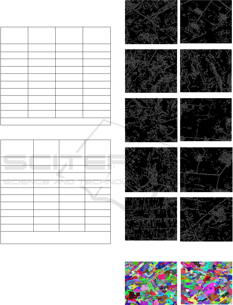
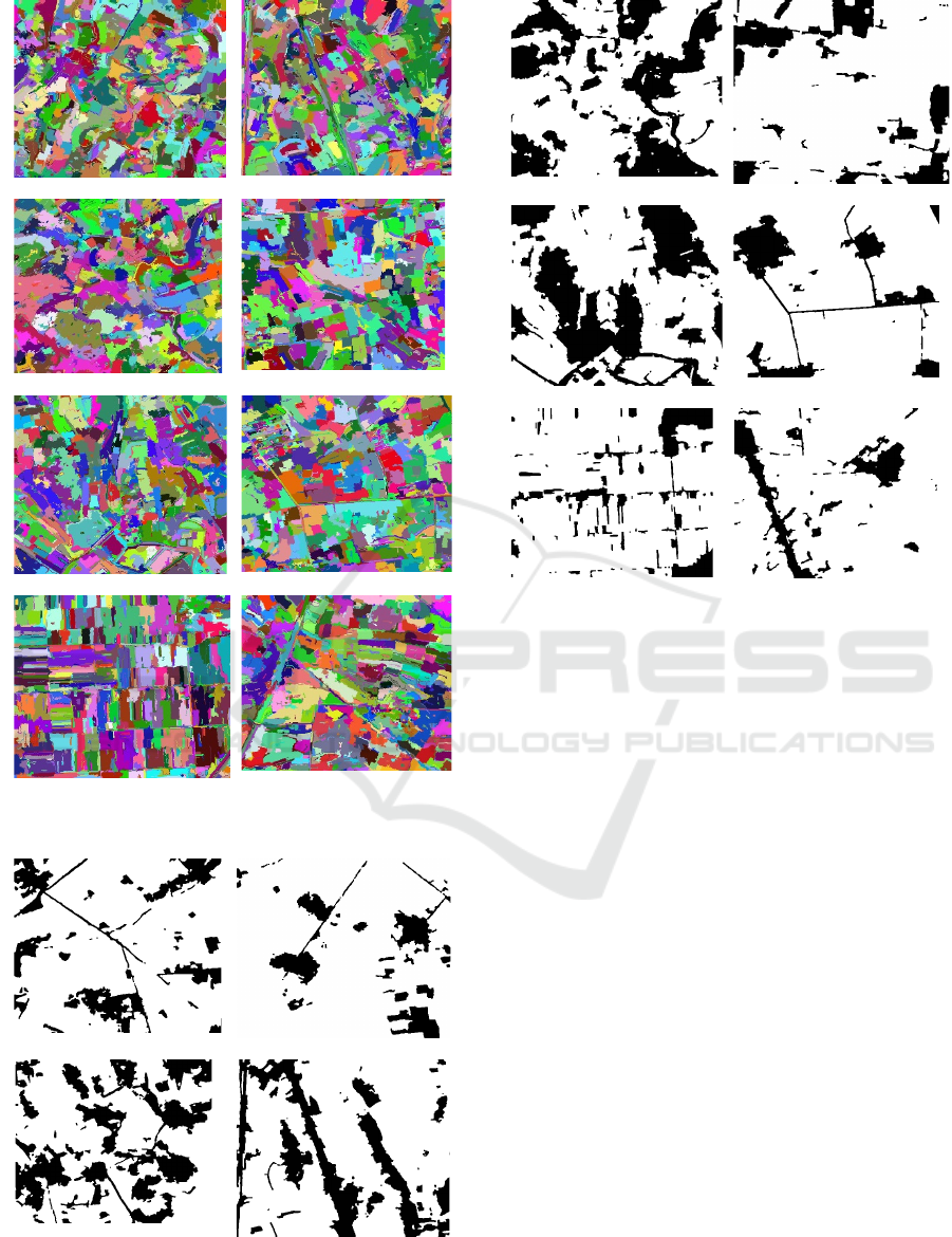
The edge detection results, image segmentation
results and the final predicted label map part of the
images during the experiment are shown in Figure 3,4
and 5.
a
)
Data1
_
cann
y
b) Data2_canny
c) Data3_cann
y
d) Data4_canny
e
)
Data5
_
cann
y
f) Data6_canny
g) Data7_cann
y
h) Data8_cann
y
i) Test1_canny
j)
Test2
_
cann
y
Figure 3: Edge detection results
a
)
Data1
_
cut
b) Data2_cut
Research on Farmland Extraction from Remote Sensing Images Based on Decision Tree
213

c) Data3_cut
d) Data4_cut
e
)
Data5
_
cut
f) Data6_cut
g) Data7_cut
h) Data8_cut
i
)
Test1
_
cut
j) Test2_cut
Figure 4: Image segmentation results
a) Data1_out
b)
Data2
_
out
c) Data3_out
d) Data4_out
e) Data5_out
f) Data6_out
g)
Data7
_
out
h) Data8_out
i) Test1_out
j)
Test2
_
out
Figure 5: Model prediction results
It is easy to see that the random forest prediction
results are much better than the decision tree, and the
results are very much as expected, the image
segmentation results are good, and the accuracy of the
labeled map is close to 90%, so the training can be
considered valid.
5 CONCLUSION
In this paper, we proposed a random forest-based
construction of multiple decision tree model to
segment and extract remote sensing image parcels for
research. Firstly, a graph theory-based segmentation
method is used for image segmentation, and the
Canny edge operator is introduced to extract edge
information, which is used to suppress the over-
segmentation phenomenon generated by it. Secondly,
it is optimized using the Bagging-based random forest
expansion algorithm. The accuracy of 88.09% was
obtained after conducting the experiment, which
gained an improvement compared with the traditional
method.
However, our method is not able to completely
distinguish all cultivated and non-cultivated land for
a single color feature, and the selected features are
only selected based on the obvious differences
ISAIC 2022 - International Symposium on Automation, Information and Computing
214

between cultivated land and other plots that are easily
recognized by the naked eye, without considering all
features, and the effect of dividing the two regions
with inconspicuous edges is not good enough, and for
the effect of dividing the region for edge detection,
the improved Canny operator or other For the
overfitting phenomenon, the overfitting can be
reduced by collecting more data sets to train the built
model, and if more rich remote sensing images are
available, the non-cultivated land can be further
divided into multi-classification problems to improve
the accuracy of the model for cultivated land
recognition.
REFERENCES
Felzenszwalb, P. F., & Huttenlocher, D. P. (2004). Efficient
Graph-Based Image Segmentation. INTERNATIONAL
JOURNAL OF COMPUTER VISION, 59(2), 167-181.
R., S., M., B., & G., L. (2018, 2018-01-01). Circular Shape
Prior in Efficient Graph Based Image Segmentation to
Segment Nucleus. Paper presented at the 2018 Digital
Image Computing: Techniques and Applications
(DICTA).
Cahuina, E. C., Cousty, J., Kenmochi, Y., Araujo, A. D.,
Camara-Chavez, G., & CENPARMI. (2018).
Algorithms for hierarchical segmentation based on the
Felzenszwalb-Huttenlocher dissimilarity
PROCEEDINGS OF THE INTERNATIONAL
CONFERENCE ON PATTERN RECOGNITION AND
ARTIFICIAL INTELLIGENCE (ICPRAI 2018) (108-
113). International Conference on Pattern Recognition
and Artificial Intelligence (ICPRAI).
Cahuina, E. C., Cousty, J., Kenmochi, Y., Araujo, A. D.,
Camara-Chavez, G., & Guimaraes, S. (2019). Efficient
Algorithms for Hierarchical Graph-Based
Segmentation Relying on the Felzenszwalb-
Huttenlocher Dissimilarity. INTERNATIONAL
JOURNAL OF PATTERN RECOGNITION AND
ARTIFICIAL INTELLIGENCE, 33(11)
Shirly, S., & Ramesh, K. (2019). Review on 2D and 3D
MRI Image Segmentation Techniques. CURRENT
MEDICAL IMAGING REVIEWS, 15(2), 150-160.
Liu, J., Yan, S., Lu, N., Yang, D., Lv, H., Wang, S., Zhu,
X., Zhao, Y., Wang, Y., Ma, Z., & Yu, Y. (2022).
Automated retinal boundary segmentation of optical
coherence tomography images using an improved
Canny operator. Scientific Reports, 12(1), 1412. http
Singh, S., Tiwari, R. K., Sood, V., Gusain, H. S., & Prashar,
S. (2021). Image Fusion of Ku-Band-Based
SCATSAT-1 and MODIS Data for Cloud-Free Change
Detection Over Western Himalayas. IEEE transactions
on geoscience and remote sensing, 60, 1-14.
Moshkov, M. (2022). On the depth of decision trees with
hypotheses. Entropy, 24(1), 116.
Wang, F., Wang, Y., Ji, X., & Wang, Z. (2022). Effective
Macrosomia Prediction Using Random Forest
Algorithm. International Journal of Environmental
Research and Public Health, 19(6), 3245.
Research on Farmland Extraction from Remote Sensing Images Based on Decision Tree
215