Integrating Machine Learning into Fair Inference

Haoyu Wang

, Hanyu Hu

, Mingrui Zhuang

and Jiayi Shen

Software School of Yunnan University, Kunming, China

The Affiliated Tianhe School of Guangdong Experimental Middle School, Guangzhou, China

Beijing NO.2 Middle School, Beijing, China

Suzhou High School, Suzhou, China

Keywords: Fairness, Machine Learning, Causal Inference, Path-Specific Effect, Natural Direct Effect, Counterfactual.

Abstract: With the boom of machine learning, fairness is an issue that needs to be concerned. The three main perspec-

tives of this paper provide a thorough look at the fairness problem: First, we introduce a handy tool for

causal inference, that is, causal graph, and apply formulas like adjustment formula, back-door formula, and

front-door formula to see the effect of interventions, which can help with the fairness. Then some approach-

es to measure the fairness are introduced: natural direct path and path-specific effect. Finally, we use coun-

terfactual inference further to study fairness with the help of causal graphs and integrate LFR, a model fo-

cusing on both group fairness and individual fairness.

1 INTRODUCTION

Nowadays, artificial intelligence is widely used in

our lives. With the increasing use of automated deci-

sion-making systems, people are concerned about

bias and discrimination in these systems. Since sys-

tems trained with the historical data will inherit the

previous biases, we need to make a fair decision so

that there are not unduly biased for or against pro-

tected subgroups in the population, such as the fe-

male, the elderly, and the ethnic minorities. The

problem is deemed as fairness in machine learning.

There are two crucial dimensions of fairness: group

fairness and individual fairness. Group fairness en-

sures that the overall proportion of members in a

protected group receiving positive or negative classi-

fication is identical to the proportion of the popula-

tion as a whole. On the other hand, individual fair-

ness achieves that any two similar individuals should

be classified similarly.

Causal inference serves as a solution to fairness.

Causality is prevalent in the universe. For example,

the cure of a disease is due to using a specific drug.

Machines can answer questions like whether this

drug should be used to make a causal inference.

Some causalities, however, may lead to discrimina-

tion on specific groups, damaging fairness. If gender

is the cause of whether he/she gets the offer, there is

no doubt that the employer biases against some par-

ticular gender, so this is unfair. In order to ensure

fairness, machine learning systems developed to

decide whether an employee can get the offer should

not consider gender.

Machines are good at predicting probability, but

it is difficult to predict results after intervening.

Counterfactual, as its name indicates, captures no-

tions of something that has not happened could hap-

pen with some conditions contrary to the fact. As a

subset of causal inference, counterfactual inference

appears to measure the fairness of machine learning

systems based on causal inference. Counterfactuals

are pretty common in our daily lives: every sentence

in the subjunctive mood can be considered a coun-

terfactual problem. When you hear your friend say-

ing, "If I had done my assignment better, I would

have got a better final score," you cannot immediate-

ly check whether this sentence is correct because

there is no easy way to find someone with the same

quality as him/her. Here "done my assignment bet-

ter" is counterfactual because "your friend" signifies

that he/she did not do homework well.

It is only recently that some researchers have

considered this issue. Several papers have aimed to

achieve group fairness, and some achieve individual

fairness. Nabi and Shpitser have considered the

problem of fair statistical inference on outcomes in a

setting where we wish to minimize discrimination

concerning a particular sensitive feature, such as

144

Wang, H., Hu, H., Zhuang, M. and Shen, J.

Integrating Machine Learning into Fair Inference.

DOI: 10.5220/0011908000003613

In Proceedings of the 2nd International Conference on New Media Development and Modernized Education (NMDME 2022), pages 144-154

ISBN: 978-989-758-630-9

 2023 by SCITEPRESS – Science and Technology Publications, Lda. Under CC license (CC BY-NC-ND 4.0)

race or gender (Nabi, Shpitser, 2018). A paper has

investigated real-world applications that have shown

biases in various ways and listed different sources of

biases that can affect AI applications (Binns 2018).

Another paper draws on existing moral and political

philosophy work to elucidate emerging debates

about fair machine learning (Mehrabi, Morstatter,

Saxena, Lerman, Galstyan, 2021). These papers

have clearly illustrated the fairness in statistical stud-

ies and even provided some application scenarios

that correlate with machine learning. However, they

do not contain a systematic approach to integrating

machine learning into the field of fairness.

The later parts of this paper are organized below:

First, we introduce a handy tool for causal inference,

that is, causal graph, and apply formulas like ad-

justment formula, back-door formula, and front-door

formula to see the effect of interventions, which can

help with the fairness. Then some approaches to

measure the fairness are introduced: natural direct

path and path-specific effect. Finally, we use coun-

terfactual inference further to study fairness with the

help of causal graphs and integrate LFR, a model

proposed by Zemel, Wu, Swersky, Pitassi, and

Dwork that focuses on both group fairness and indi-

vidual fairness (Zemel, Wu, Swersky, Pitassi,

Dwork, 2013). All the theories and experiments are

based on the Community and Crime Dataset from

the UCI repository (Acharya, Blackwell, Sen, 2016).

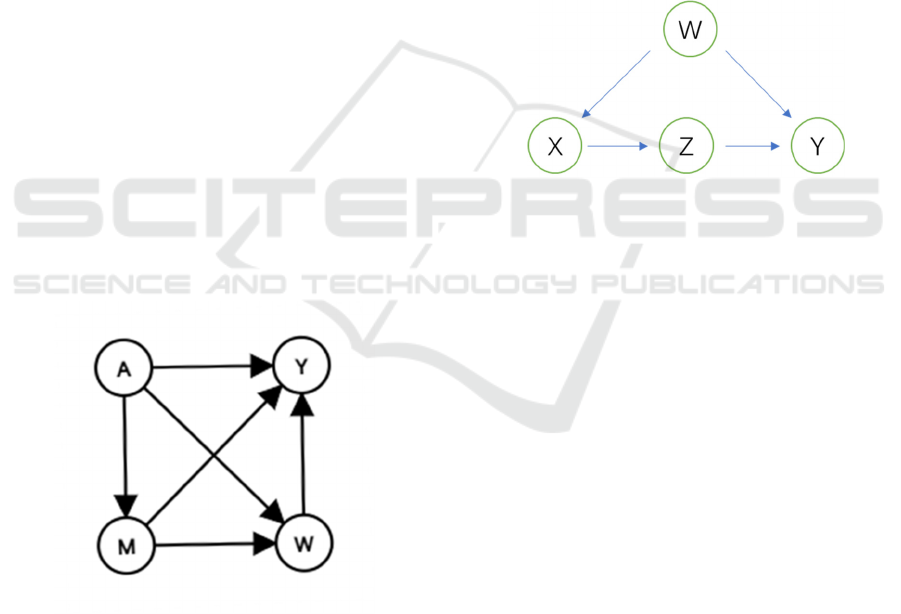
2 CAUSAL GRAPHS AND

CAUSAL INFERENCE

2.1 Introduction to Causal Graphs

Causal graphs can be used in describing the causal

relationship between attributes. As a visual model of

causality between variables in a system, the causal

graph makes it easier to draw realistic causal infer-

ences, like doing exercises “causes” lower blood

pressure. It plays a role by stimulating the identifica-

tion of more potential confounding factors and the

source of selection bias.

A causal graph is a directed acyclic graph

(DAG), including a collection of nodes (also re-

ferred to vertices on some occasions) and directed

edges. So the graph can be represented by 𝐺=

{𝑁,𝐸}, where 𝑁 is the set of nodes and 𝐸 is the set

of edges. An example of a causal graph is shown as

Fig. 1:

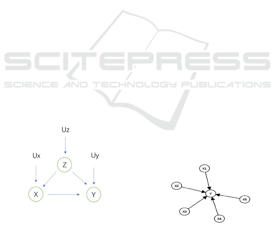
Figure 1: An example of a causal graph

In Fig. 1, we see that

𝑁=

{

𝐴,𝑀,𝑊,𝑌

}

(1)

𝐸=

{

(

𝐴,𝑀

)

(

𝐴,𝑊

)

(

𝐴,𝑌

)

(

𝑀,𝑊

)

(

𝑀,𝑌

)

(

𝑊,𝑌

)

}

(2)

Each node in the graph represents a variable. We

use solid nodes to represent observed variables and

dashed nodes to represent unobserved variables. An

edge indicates the causal effect between two varia-

bles, like (𝐴,𝑀), the edge directing from 𝐴 to 𝑀,

which means that 𝐴 is the “cause” of 𝑀. Here we

also say 𝐴 is the parent node of 𝑀. Two nodes are

adjacent if they are connected by an edge. There are

paths between 2 nodes if they are connected by some

sequences of edges. For example, 𝐴 and 𝑌 are adja-

cent. From 𝐴 to 𝑊, there are 2 paths: 𝐴→𝑊, 𝐴→

𝑀→𝑊.

2.2 The Crime Dataset and Our Causal

Graphs

In later parts of this paper, experiments are conducted

on the Community and Crime Dataset, retrieved from

the UCI repository (Acharya, Blackwell, Sen, 2016).

Later we will call it Crime Dataset for short. It con-

tains 1994 samples, and each of them contains 128

attributes. The first 4 attributes are state, county,

community, communityname, which are nominal

data, serving as the identifier of the sample and not

for prediction. The 5

attribute is fold, whose values

are integers ranging from 1 to 10, used for 10-fold

cross validation. The 6

to the 127

attributes are

social and socio-economic data that is plausible to do

with the crime rate, such as PolicPerPop (police

officers per 100K population). The last attribute is

the goal attribute to be predicted: Violent-

CrimesPerPop (total number of violent crimes per

Integrating Machine Learning into Fair Inference

145

100K population).

It is worth noting that the values of the 6

to the

128

attributes have been normalized into the deci-

mal range from 0.00 to 1.00, using an unsupervised,

equal-interval binning method. In this way, attributes

retain their distribution and skew (for example, the

population attribute has a mean value of 0.06 because

most communities are small). The normalization

preserves rough ratios of values within an attribute.

The dataset we used combines socio-economic

data, law enforcement, and crime data from the 1990

U.S. Census. Data is described based on original

values and used to predict the crime rate of specific

communities in the United States. Besides, there are

some sensitive attributes in the data about age, gen-

der, and race in this dataset. For our goal of fairness,

we try not to let these sensitive attributes decide the

crime rate. However, it is inevitable to use these

attributes for some causal inferences of other non-

sensitive attributes.

For later experiments, we have drawn some caus-

al graphs based on the Crime Dataset. They are

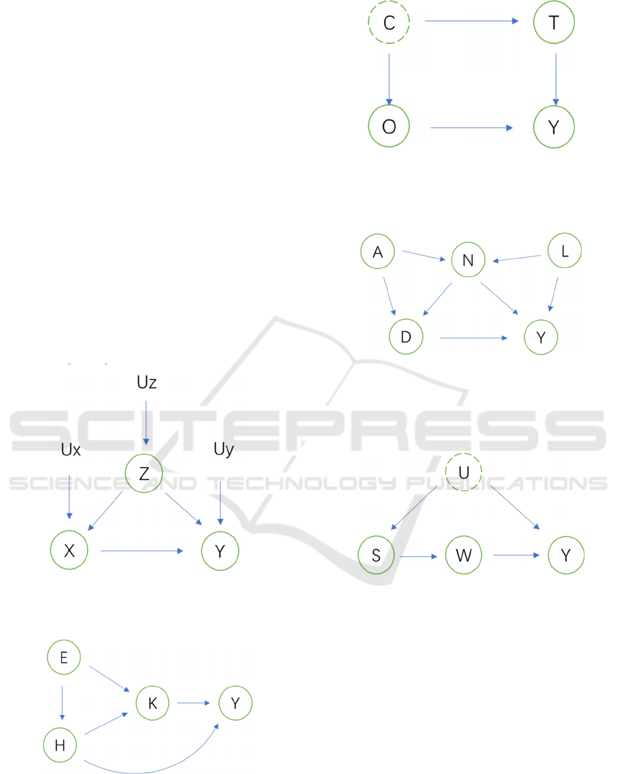
shown as Fig. 2-Fig. 6:

Figure 2: Causal Graph 1. X denotes the per capita in-

come; Z denotes the percentage of people 16 and over who

are employed; Y denotes the crime rate.

Figure 3: Causal Graph 2. H denotes percentage of people

25 and over with a bachelors degree or higher education; E

denotes percent of people who do not speak English well;

K denotes percentage of households with wage or salary

income in 1989; Y denotes the crime rate.

Figure 4: Causal Graph 3. O denotes the police operating

budget; C denotes the commodity prices (unobserved); T

denotes the percent of people using public transit for

commuting; Y denotes the crime rate.

Figure 5: Causal Graph 4. A denotes percentage of kids

born to never married; N denotes percentage of population

who are divorced; L denotes percentage of people under

the poverty level; D denotes percent of housing occupied;

Y denotes the crime rate.

Figure 6: Causal Graph 5. S denotes number of different

kinds of drugs seized; U - percent of people using drugs

(unobserved);

2.3 Interventions on Causal Graphs

The ultimate goal of many statistical studies is to

predict the effect of interventions. For example, we

collect data on car accidents to find intervention

factors to reduce the occurrence of car accidents;

when we study new drugs, we intervene by asking

patients to take drugs and observe the reaction of

patients after taking drugs. When randomized con-

trolled trials are not feasible, we often implement

observational studies to obtain the relationship be-

tween variables by controlling specific data.

Through this intervention, we can block the causal

NMDME 2022 - The International Conference on New Media Development and Modernized Education

146

relationship between some variables and analyze the

impact of other variables.

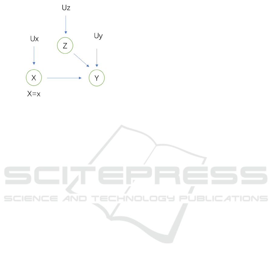
Figure 7: Causal Graph 1 after the intervention on X

In the case of Fig. 2, in order to determine the ef-

fect of 𝑋 on 𝑌, we simulate the intervention in the

form of a graph surgery (as in Fig. 7 above, where 𝑋

is controlled to be 𝑥, the manipulated probability is

𝑃



. In the manipulated model of Fig. 7, the causal

effect 𝑃(𝑌 = 𝑦|𝑑𝑜(𝑋 = 𝑥)) is equal to the condi-

tional probability 𝑃



(𝑌=𝑦|𝑋=𝑥). Combined with

the primary attributes of probability and variables,

we get a causal effect formula expressed by pre-

intervention probability, known as adjustment formu-

la：

𝑃

(

𝑌=𝑦

𝑑𝑜(𝑋 = 𝑥))

= 𝑃

(

𝑌=𝑦

𝑋 = 𝑥, 𝑍 = 𝑧) 𝑃(𝑍



=𝑧)

(3)

There is another application of adjustment formu-

la in Fig. 3. We want to gauge the effect of higher

education (H) on crime rate (Y). We assume that

people who have income are less likely to commit

crimes. Using the same method as shown in (1), we

get the following formula: is shown as belows

𝑃

(

𝑌=𝑦

𝑑𝑜(𝐻 = ℎ)) = 𝑃

(

𝑌=𝑦

𝐻 = ℎ, 𝐾 = 𝑘)



𝑃

(

𝐾=𝑘, 𝐸=𝑒, 𝐻=ℎ

)

𝑃

(

𝑍=𝑧

)



(

)

In the above discussion, we concluded that we

should adjust for a variable's parents when we are

trying to determine its effect on another variable.

Nevertheless, often the variables have unobserved or

inaccessible parents. In those cases, we use a simple

test called the back-door criterion: given an ordered

pair of variables (𝑋,𝑌) in a directed acyclic graph 𝐺,

a set of variables 𝑍 satisfies the back-door criterion

relative to (𝑋,𝑌) if no node in 𝑍 is a descendant of

𝑋, and 𝑍 blocks every path between 𝑋 and 𝑌 that

contains an arrow into 𝑋. If a set of variables 𝑍 satis-

fies the back-door criterion for 𝑋 and 𝑌, then the

causal effect of 𝑋 on 𝑌 is given by the back-door

formula:

𝑃

(

𝑌=𝑦

𝑑𝑜(𝑋 = 𝑥))

= 𝑃

(

𝑌=𝑦

𝑋 = 𝑥, 𝑍 = 𝑧) 𝑃(𝑍 = 𝑧)



(

)

In Fig. 4, we are trying to gauge the effect of a

police operating budget (O) on crime rate (Y). We

have also measured people for public commuting

(T), which has an effect on the crime rate. Further-

more, we know that commodity prices (C) affect

both 𝑂 and 𝑇, but it is an unobserved variable. In-

stead, we search for an observed variable that fits the

back-door criterion from 𝑂 to 𝑌. We find that 𝑇,

which is not a descendant of 𝑂, also blocks the back-

door path 𝑂←𝐶→𝑇→𝑌. Therefore, W meets the

back-door criterion. By using the adjustment formu-

la, we got the following formula:

𝑃

(

𝑌=𝑦

𝑑𝑜(𝑂 = 𝑜)) =

𝑃

(

𝑌=𝑦

𝑂 = 𝑜, 𝑇 = 𝑡) 𝑃(𝑇 = 𝑡)



(

)

Do operation can also be applied to some graph

patterns that do not meet the back-door criterion to

determine the causal effect that seems to have no

solution at first. One such pattern, front-door, can

identify the causal effect shown in Fig. 6, where the

variable U is unobserved and hence cannot be used to

block the back-door path from X to Y. A set of vari-

ables Z is said to satisfy the front-door criterion rela-

tive to an ordered pair of variables (𝑋,𝑌) if

1. Z intercepts all directed paths from X to Y.

2. There is no unblocked path from X to Z.

3. All back-door paths from Z to Y are blocked

by X

This method can identify the causal effect in Fig.

6 through two consecutive applications of the back-

door path. First, there is no back-door path from S to

W. so we can immediately write the effect of S on W

𝑃

(

𝑊=𝑤

)

𝑑𝑜

(

𝑆=𝑠

)

 = 𝑃

(

𝑊=𝑤

𝑆=𝑠

)

7

then, the back-door path from W to Y, namely 𝑊←

𝑆←𝑈→𝑌, can be blocked by conditioning on X so

that we can write the second formula like this

𝑃

(

𝑌=𝑦

𝑑𝑜

(

𝑊=𝑤

)

=𝑃

(

𝑌=𝑦

𝑆 = 𝑠, 𝑊 = 𝑤) 𝑃(𝑆 = 𝑠)



(8)

Integrating Machine Learning into Fair Inference

147

Now we chain together the two partial effects to

obtain the overall effect of X on Y by summing all

states' smaller z of capital Z, and we can get this.

Through some changes in expression, we finally get

the impact of the number of drugs on the crime rate.

𝑃

(

𝑌=𝑦

𝑑𝑜

(

𝑆=𝑠

)

) =





𝑃

(

𝑌=𝑦

𝑑𝑜(𝑊 = 𝑤))𝑃

(

𝑊=𝑤

𝑆 = 𝑠) 9

2.4. Calculating the Interventions

Some formulas are deducted, though, yielding their

values is another problem. In Crime Dataset, all the

data for prediction and the outcome is continuous,

which means that the probability with variables con-

ditional on fixed values is insignificant. Also, it

seems impossible to calculate the probability of a

variable fixed on an exact value—instead, expecta-

tion matters. Nevertheless, machine learning and

statistics help.

Let us start with an example: the formula for Fig.

𝑃

(

𝑌=𝑦

𝑑𝑜(𝑋 = 𝑥))

= 𝑃

(

𝑌=𝑦

𝑋 = 𝑥, 𝑍 = 𝑧) 𝑃(𝑍 = 𝑧)



10

Since 𝑃(𝑌 = 𝑦) is hard to get, we convert it to

𝔼𝑌𝑑𝑜

(

𝑋=𝑥

)

=𝔼



(

𝑌

𝑋=𝑥,𝑍=𝑧

)

𝑃

(

𝑍=𝑧

)

(11)

In order to learn the effect on Y when we inter-

vene X, we get the formula above based on the ad-

justment formula. Since Z is continuous,



𝔼

(

𝑌

𝑋 = 𝑥, 𝑍 = 𝑧) 𝑃(𝑍 = 𝑧)



can be further

converted to formulas with expectation. With the

preliminary 𝑋 = 𝑥

the formula means “given 𝑋=𝑥

and a random selected 𝑍, the expectation of 𝑌”, that

is:

𝔼𝑌𝑑𝑜

(

𝑋=𝑥

)

=𝔼



(

𝑌

𝑋=𝑥,𝑍=𝑧

)

𝑃

(

𝑍=𝑧

)

=𝔼

(

𝑌

𝑋=𝑥,𝑍

)

=𝔼

(

𝑌

𝑋=𝑥

)

𝔼

(

𝑍

)(

)

To get the expectation 𝔼(𝑌|𝑋 = 𝑥), we can train

a model using the samples in the dataset that predicts

𝑌 with 𝑋. Amazingly, among many machine learning

models, it is linear regression that best fit the causal

relation from 𝑋 to 𝑌. The result of the prediction is

shown in Fig. 8.

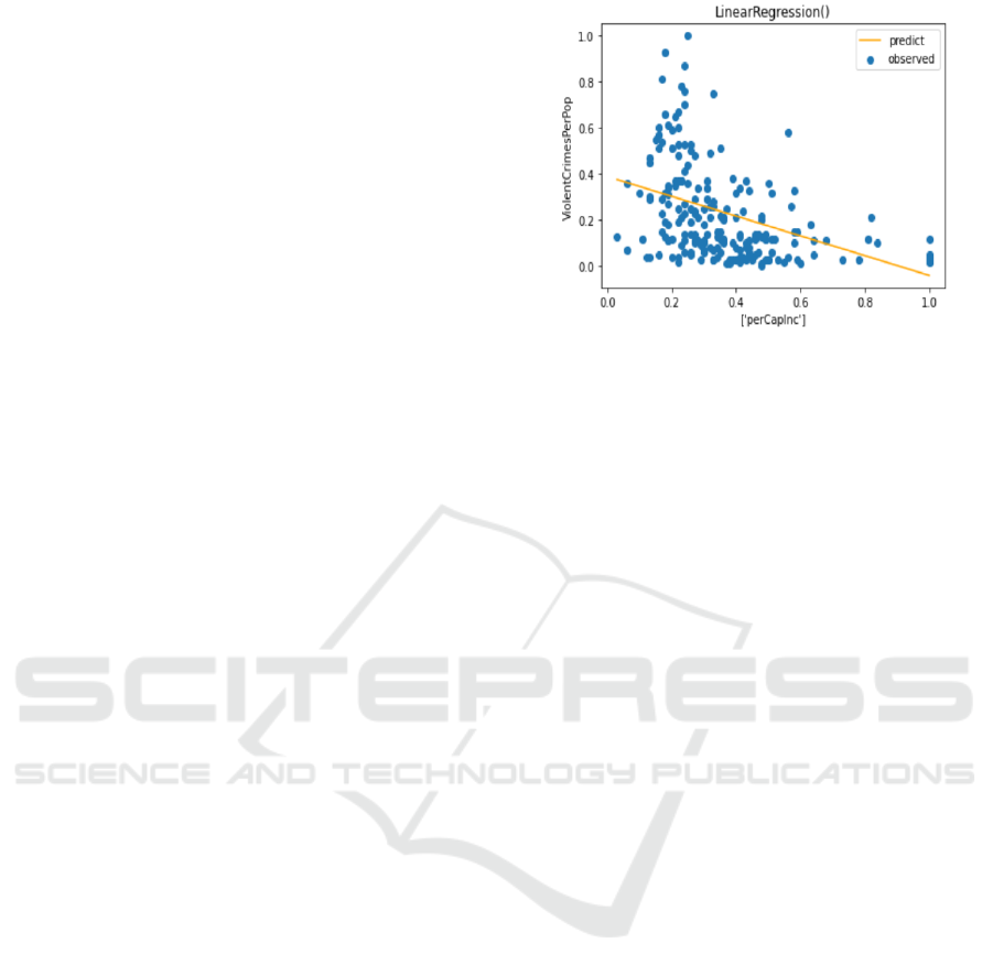
Figure 8: Diagram of the best model using perCapInc to

predict ViolentCrimesPerPop

Assume that we are interested in

𝔼𝑌𝑑𝑜

(

𝑋=0.5

)

, then we input 𝑋=0.5 and get

predicted value 0.175 , so 𝔼𝑌𝑑𝑜

(

𝑋=0.5

)

=

0.175. 𝔼(𝑍) can be simply computed using the sam-

ples in the dataset, which is 0.501. As a result:

𝔼𝑌𝑑𝑜

(

𝑋=0.5

)

=𝔼



(

𝑌

𝑋=0.5,𝑍=𝑧

)

𝑃

(

𝑍=𝑧

)

=𝔼

(

𝑌

𝑋=0.5,𝑍

)

=𝔼

(

𝑌

𝑋=0.5

)

𝔼

(

𝑍

)

= 0.175  0.501 = 0.088

(

)

The result indicates that, after exerting interven-

tion 𝑑𝑜

(

𝑋=0.5

)

, 𝑌 is expected to be 0.088.

Formulas on other graphs can also be computed

this way. The approach of computing intervention on

continuous data is concluded as:

 Express the 𝑃(𝑌 = 𝑦|𝑑𝑜(𝑋 = 𝑥)) by expres-

sions without 𝑑𝑜, using adjustment formula, back-

door formula, front-door formula, and so on.

 Convert the probability expression to expecta-

tion, like 𝑃(𝑌 = 𝑦) to 𝔼(𝑌)

 Calculate/Predict the 𝔼:

 The expectation of a single variable is the mean

value of this variable in the dataset

 For the expectation of compound expression

like 𝔼(𝑌|𝑋 = 𝑥), build a model predicting 𝑌 using

𝑋, then input 𝑋=𝑥 and use the predicted value

3 MEASURING THE FAIRNESS

3.1 Mediation and Direct Paths

Under some circumstances, we concentrate on the

effect of one variable 𝑋 on another variable 𝑌 in

causal graphs. There may be many paths from 𝑋 to

𝑌, and some are direct while some are not. So the

effect of 𝑋 to 𝑌 includes the direct effect and the

NMDME 2022 - The International Conference on New Media Development and Modernized Education

148

indirect effect.

Mediation is encoded via a counterfactual con-

trast using a nested potential outcome of the form

𝑌(𝑎,𝑀(𝑎



)) (Nabi, Shpitser, 2018). Then a treat-

ment like 𝑋=𝑎 can be divided into two disjoint

parts: one acts on 𝑌 but not 𝑀, and the other acts on

𝑀 but not 𝑌. Later, we will mainly focus on the for-

mer one, that is, the direct effect.

3.2 Natural Direct Effect

In causal mediation analysis, one quantity of interest

is the natural direct effect (NDE). It is the impact of

altering treatment underneath it while fixing the

mediator to its unit-specific plausible value. The

NDE compares the mean outcome, which is only

directly influenced by the part of the treatment that

will exert an effect on it, with the one under the

placebo treatment (Binns 2018). Given 𝑌(𝑎,𝑀(𝑎



)),

we define the following effects on the mean differ-

ence scale: the natural direct effect as

𝔼𝑌(𝑎,𝑀(𝑎



))  𝔼𝑌(𝑎



)

which means for the outcome 𝑌, 𝐴 is set to 𝑎, and 𝑀

is set to the value when 𝐴 is set to 𝑎



3.3 Path-specific Effect

Path-specific effect (PSE) is a crucial indicator for

evaluating mediation in the presence of multiple

intermediaries.

Figure 9: An example of a causal graph

From the graph Fig. 9, we can see there are four

ways to go from 𝐴 to 𝑌: 𝐴→𝑌,𝐴→𝑊→𝑌,𝐴→

𝑀→𝑌,𝐴→𝑀→𝑊→𝑌. If we wish to evaluate

the contribution of 𝐴→𝑊→𝑌, with the presence

of 𝐴→𝑌, and 𝐴→𝑀→𝑊→𝑌, effects along the

path 𝐴→𝑊→𝑌 is known as Path-specific effect.

On the path of interest, 𝐴 is set to the value 𝑎, and

on other paths, 𝐴 is set to the baseline value 𝑎



. With

the concept, the path-specific effect from 𝐴 to 𝑌

along the path 𝐴→𝑊→𝑌 can be formulated by

𝔼𝑌(𝑎



,𝑊(𝑀(𝑎



),𝑎),𝑀(𝑎



))  𝔼𝑌(𝑎



)

We formalize the existence of discrimination as

the existence of a particular path-specific effect. The

reason why we use PSE is that when problems arise,

such as gender or racial discrimination, we can issue

conceptualization, make causal graphs according to

the problems, and define a fair path from 𝐴 (attribute

about gender/race) to the outcome 𝑌 (crime rate),

may be related to some media, or it is a direct-effect

path, the problem will increase the PSE along these

paths.

3.4 Using PSE in Our Graphs

Figure 10: A causal graph we use to study the PSE. W

denotes the percentage of people living in areas classified

as urban; X denotes the percentage of the population that

is African American; Z denotes median household in-

come; Y denotes crime rate.

First, we focus on the causal graph Fig. 10.

It is inevitable to encounter sensitive variables in

various data. When we find some paths that may be

unfair, we can take some measures to avoid them.

When we use Fig. 10 to estimate the impact of the

variables on the crime rate, we may come to some

discriminatory conclusions: the increase of African

American income will reduce the crime rate. Obvi-

ously, the logical relationship between these two

things is unfair. We will avoid this discrimination by

choosing other paths or increasing fairness. This is

where PSE works.

The path we are interested in is 𝑊→𝑌.

PSE: 𝔼𝑌

(

𝑤

)

 𝔼𝑌(𝑤,𝑍(𝑋(𝑤′),𝑤),𝑋(𝑤′))

As 𝑊 is set to the baseline 𝑤



, 𝑋 is represented

with 𝑋(𝑤



), 𝑍 is represented with 𝑍(𝑋(𝑤



),𝑤), and

𝑌 is 𝑌(𝑤,𝑋(𝑤



),𝑍(𝑋(𝑤



),𝑤



)). Changing the 𝑤



𝑤, since the baseline value will not have a great

influence on the values we care about, so 𝑋 is repre-

sented with 𝑋(𝑤) , 𝑍 is represented with

𝑍(𝑋(𝑤



),𝑤), and 𝑌 is 𝑌(𝑤,𝑋(𝑤



),𝑍(𝑋(𝑤



),𝑤)).

Then we focus on another causal graph, above

Integrating Machine Learning into Fair Inference

149

mentioned Fig. 3.

The path we are interested in is 𝐸→𝐻→𝐾→𝑌.

PSE: 𝔼𝑌(𝑒,𝐻(𝑒



),(𝐾(𝐻(𝑒



),𝑒)) 

𝔼𝑌(𝑒,𝐻(𝑒



),𝑒)

Since we want to evaluate the contribution on

𝐸→𝐻→𝐾→𝑌, with the presence of 𝐸→𝐾→𝑌,

and 𝐸→𝐻→𝑌, effects along the path 𝐸→𝐻→

𝐾→𝑌 is actually the path-specific effect. As 𝐸 was

set to the baseline value 𝑒



, since baseline value will

not affect the value of the path we are interested in,

𝐻 will be represented with 𝐻(𝑒



4 COUNTERFACTUAL

INFERENCE

4.1 Introduction to Counterfactual

Inference

Unlike the formulas introduced in the last sessions,

which focus on the whole dataset with a large num-

ber of samples, the counterfactual inference is the

study of the counterfactual effect of a single sample.

But some preliminary to computing the counterfac-

tual depends on the whole dataset, also.

In accord with Chapter 4 of Causal Inference in

Statistics: a Primer (Pearl, Glymour, Jewell, 2016),

we define 𝑌



(𝑢) = 𝑦 as “𝑌 would be 𝑦 if 𝑋 was 𝑥,

with 𝑢

→

=𝑢” where 𝑢

→

is the vector of exogenous

variables, like {𝑢



,𝑢



,𝑢



} in this example. Assume

that "your friend" had put 1.5 times of energy into

the assignment. The answer to the grade example

can be denoted as 𝑌

.

(𝑢



,𝑢



,𝑢



). Here

𝑋,𝑌,𝑍

are given, through which we can calculate 𝑢



,𝑢



,𝑢



Figure 1: A causal graph of the grade example. Z: assign-

ment; X: performance score; Y: final score

According to Fig. 11 which describes the coun-

terfactual problem at the beginning, that your friend

saying, “If I had done my assignment better, I would

have got a better final score”, we see that assignment

can affect the grades both directly and indirectly. To

quantify the effects, we assume that:

𝑍=𝑢



(

)

𝑋=2𝑍+𝑢



(

)

𝑌=𝑋+3𝑍+𝑢



(

)

For the sample of “your friend” in the example,

assume that 𝑍 = 1,𝑋 = 3,𝑌 = 5, we can substitute

these values into the equations above and yield 𝑢



1,𝑢



=1,𝑢



=1 . The answer became

𝑌

.

(1,1,1) . If 𝑍=1 was replaced with 𝑍=

1.5, then:

𝑋=2𝑍+𝑢



=21.5+1=4

(

)

𝑌=𝑋+3𝑍+𝑢



=5+31.51=8.5

(

)

Since 𝑌 would be 8.5 if 𝑍 was modified to 1.5,

we can conclude that the final score of "your friend"

would gain a 70% increase if he/she had put 1.5

times of energy into the assignment. In other words,

after exerting a counterfactual effect,

𝑌

.

(

1,1,1

)

=8.5, while 𝑌=5 originally.

In later parts, we will discuss some approaches to

compute the counterfactual based on some chosen

attributes in Crime Dataset, then model the relations

between them.

4.2 Model the Relations Using Machine

Learning Methods

In causal graphs, each edge can be regarded as a

relation between two variables. For a node 𝑌 in the

graph with its parent nodes being 𝑋



,𝑋



,⋯,𝑋



(in

other words, for each integer 𝑖 satisfying 𝑖∈1,𝑛,

there is an edge from 𝑋



to 𝑌), the relations can be

modeled as 𝑌=𝑓



(𝑋



,𝑋



,⋯,𝑋



) . If exogenous

variable 𝑢



is into consideration, the equation will

become 𝑌=𝑓



(

𝑋



,𝑋



,⋯,𝑋



)

+𝑢



. For example,

on condition that 𝑛=5, the relation among

𝑋



,𝑋



,𝑋



,𝑋



,𝑋



and 𝑌 is illustrated as Fig. 12.

Figure 12: An example of such causal graphs: 𝑛=5, and

each of 𝑋



,𝑋



,⋯,𝑋



directs to 𝑌. In this situation, we

represent 𝑌 as 𝑌=𝑓



(

𝑋



,𝑋



,⋯,𝑋



)

+𝑢



NMDME 2022 - The International Conference on New Media Development and Modernized Education

150

Although counterfactual inference focuses on the

effect of a single sample, a large amount of samples

in the dataset is required to train the models. When

modeling the relations, exogenous variables like

𝑢



,𝑢



can be seen as the noise with a mean of 0.

However, when computing the outcome with coun-

terfactual assumptions, exogenous variables differ in

different samples, which will be discussed in 4.3.

The simplest way to model the function is as-

suming they are linearly correlative: 𝑌=𝑎



𝑋



𝑎



𝑋



+⋯+𝑎



𝑋



+𝑢



, like the example in 4.1.

However, as we plot the relations between two vari-

ables, it is clear that the linear model cannot best fit

the relation, which leads to a relatively high bias, as

Fig. 13 shows.

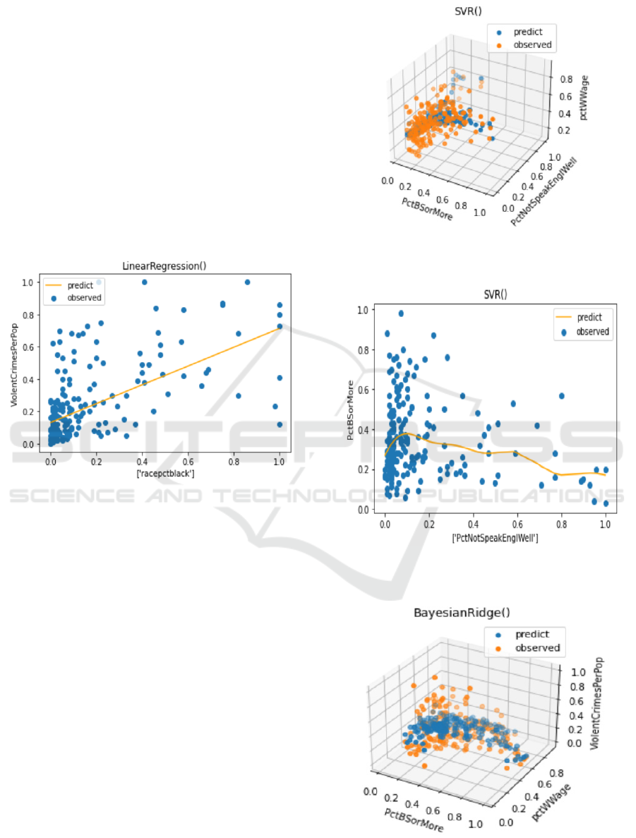
Figure 13: Adoption of linear regression on two attributes

on Crime Dataset: X-axis is racepctblack (percentage of

African Americans) and Y-axis is ViolentCrimesPerPop

(total number of violent crimes per 100K population)

In our causal graphs with attributes from Crime

Dataset, we tested 4 different machine learning

models: Linear Regression, Decision Tree, Support

Vector Regression, and Bayesian Ridge. For each

model, we trained it using 10-fold cross validation,

which provides a reasonable assessment of the per-

formance of the model. Then we select the best

model for each causal function according to the min-

squared error (MSE) of the prediction. The function

is represented as a node, all its parent nodes and the

edges between them in the causal graph.

Take the causal graph Fig. 3 as an example. The

results of model fitting are shown in Fig. 14-Fig. 16.

Figure 14: Scatter diagram of the best model using PctB-

SorMore, PctNotSpeakEnglWell to predict pctWWage

Figure 15: Diagram of the best model using PctNotSpeak-

EnglWell to predict PctBSorMore

Figure 16: Scatter diagram of the best model using PctB-

SorMore, pctWWage to predict ViolentCrimesPerPop

Integrating Machine Learning into Fair Inference

151

From the results, we find that SVR (support vec-

tor regressor) best fits the former two relations,

while bayesian ridge best fits the last relation. The

other graphs are conducted the same things. We save

the best models and apply them in later steps of

counterfactual inference.

4.3 Compute the Counterfactuals

Chapter 4 of Causal Inference in Statistics: a Primer

(Pearl, Glymour, Jewell, 2016) indicates that there

are 3 steps to compute the counterfactual. Combined

our work with the illustration of the book, we con-

clude that our steps are:

 Abduction: Use evidence of an actual sample to

determine the value of exogenous variables 𝑈;

 Action: substitute the equations for the goal at-

tribute 𝑌 with the interventional values 𝑋=𝑥, result-

ing in the modified set of equations 𝑌



(𝑈);

 Prediction: compute the implied distribution on

attributes except 𝑋 based on 𝑈 and models built in

the last session, then the predicted value 𝑌

can repre-

sent 𝑌



(𝑈).

Our experiment focused on causal graph Fig. 10,

manually selecting a community called Bethle-

hemtownship from Crime Dataset. Its values are

{𝑊 = 0.43,𝑋 = 0.02,𝑍 = 0.50,𝑌 = 0.03} . We

exerted counterfactual effect 𝑋=0.23, since 𝑋 de-

notes the percentage of the population that is African

American with its 75% quantile being 0.23. By

computing 𝑌

.

(𝑈), that is, "what if there were

more African Americans in this community" we can

judge whether the models trained in 4.2 discriminate

against the specific race.

Table 1. Result of the counterfactual experiment

X W Z Y

Original

sample

0.02 0.43 0.50 0.03

Sample after

counterfactual

effec

0.23

(presupposed)

0.43

(original)

0.29 0.17

According to Table 1 showing the results, we can

say that, unfortunately, the models we trained are

unfair. Since we simply adjust 𝑋 with 𝑊 unaltered,

the predicted crime rate increased significantly. It is

worth noting that mediator 𝑍 changes as well, which

suggests that it is already unfair halfway to the out-

come variable. But there are ways to tackle this

problem, such as LFR introduced in the next session.

4.4 Application of Learning Fair

Representations in Counterfactual

Inference

Learning fair representations, abbreviated to LFR, is

a machine learning-based model which takes fair-

ness into consideration, both group fairness and

individual fairness while assuring the accuracy of

prediction at the same time (Zemel, Wu, Swersky,

Pitassi, Dwork, 2013). LFR works on the dataset that

is divided into protected group and unprotected

group, and then it tries to attain the group fairness

between the two groups.

To integrate LFR in our experiment for a predic-

tion with better fairness, we adopted the criterion of

LFR, that is:

𝐿=𝑎



𝐿



+𝑎



𝐿



+𝑎



𝐿



(

)

In this formula, 𝑎



,𝑎



,𝑎



are hyperparameters

mastering the tradeoff among 𝐿



,𝐿



,𝐿



, which are

three disparate measurements to be minimized: 𝐿



measures the gap between the protected group and

unprotected group in the prediction; 𝐿



means the

information loss in the prediction; 𝐿



scales how

inaccurate the prediction is, so the lower 𝐿



is, the

more accurate the model predicts. The detailed cal-

culation of 𝐿



,𝐿



,𝐿



is illustrated in Learning fair

representations (Zemel, Wu, Swersky, Pitassi,

Dwork, 2013).

For a node 𝑌 in our causal graph with parent

nodes 𝑋



,𝑋



,⋯,𝑋



, if 𝑋



is a sensitive attribute,

then we separate protected and unprotected groups

depending on the value of 𝑋



, and train an LFR

model to fit 𝑌=𝑓



(

𝑋



,𝑋



,⋯,𝑋



)

In our experiment, including some sensitive at-

tributes, like the one in 4.3 on Fig. 10, we can excep-

tionally adopt LFR on unfair paths, while fair paths

are simply assembled the best model selected in 4.2.

In this experiment, we adopted LFR on 𝑋→𝑍, and

the results are shown as below:

Table 2. Result of the counterfactual experiment, using

LFR on 𝑋→𝑍

X W Z Y

Original

sample

0.02 0.43 0.50 0.03

Sample after

counterfactual

effec

0.23 (presup-

posed)

0.43

(original)

0.29 0.17

Sample after

counterfactual

effect (using

LFR on

𝑋

→

𝑍)

0.23 (presup-

posed)

0.43

(original)

0.39 0.05

NMDME 2022 - The International Conference on New Media Development and Modernized Education

152

Comparing the prediction of counterfactual ef-

fect by models integrating LFR and the prediction

with no concern on fairness (see Table 2), it is ex-

plicit that LFR makes it a little fairer since 𝑍 (medi-

an household income) predicted by 𝑋 is not that low.

The outcome 𝑌 (total number of violent crimes per

100K population) is relatively low.

Moreover, we notice that the adopting LFR on

𝑋→𝑍 makes predicted 𝑍 above its average of 0.36.

If we divide the dataset into the protected group and

unprotected group according to 𝑋 (samples with 𝑋>

0.23 is divided into the protected group), we see that

the mean of 𝑍 in the protected group is 0.24 (below

the average), while the value in unprotected group is

0.40 (above the average). The predicted 𝑍 using

LFR, interestingly, is close to 0.40.

5 CONCLUSION

In this paper, we took fairness in machine learning

as a starting point since it became a social issue

today. We chose Community and Crime Dataset

because it has lots of attributes, including some sen-

sitive ones, and we conducted experiments on it to

explore some approaches to improve fairness. Our

research was a glimpse of the world of fairness from

three different perspectives.

In causal inference, we focused on the effect of

intervening some variables on the outcome variable,

which we denote as 𝑃(𝑌 = 𝑦|𝑑𝑜(𝑋 = 𝑥)), inspired

by some previous work (Binns 2018). Since the

effect of intervention is not observable, we need to

convert expression with 𝑑𝑜 to probability condition-

al on observable variables. The adjustment formula,

back-door formula, and front-door formula are of

great importance.

However, the dataset we chose contains mostly

continuous data, making the probability of a con-

crete point meaningless. In our research, we innova-

tively proposed an approach that replaces 𝑃 with 𝔼,

the expectation. For example, 𝑃(𝑌 = 𝑦|𝑑𝑜(𝑋 = 𝑥))

is equivalent to 𝔼𝑌𝑑𝑜

(

𝑋=𝑥

)

. Then by either

calculating directly or predicting with machine

learning models, we can get the expectation of 𝑌

while intervening on 𝑋.

Later, we apply some measurements for fairness

on our dataset: natural direct path and path-specific

effect, proposed by Nabi and Shpitser (Nabi, Shpit-

ser, 2018). They work when there are multiple paths

from 𝑋, the variable we are interested in, to 𝑌, the

outcome variable. By shadowing the mediators be-

tween 𝑋 to 𝑌, we can learn the effect of 𝑋 to 𝑌 spe-

cific to certain fair paths. For example, it is unfair to

make gender directly affect the offer, but it is fair

that gender influences the capabilities concerning

the offer.

Finally, we studied the counterfactual inference.

The goal of this part is computing 𝑌



(𝑢), which

means the value 𝑌 would be if 𝑋 was 𝑥, with exoge-

nous variables 𝑈=𝑢. The first step is to build mod-

els for edges in causal graphs, which signify the

causal relationship between variables. We tried 4

different machine learning models: Linear Regres-

sion, Decision Tree, Support Vector Regression, and

Bayesian Ridge, and trained each of them by 10-fold

cross validation. Then we computed the counterfac-

tual effect, according to the approaches introduced

in Chapter 4 of Causal Inference in Statistics: a

Primer (Pearl, Glymour, Jewell, 2016).

Since we found that building the models as men-

tioned above without concern on fairness may lead

to discrimination on certain protected groups, we

introduced learning fair representations to improve

fairness. This model performs well on both group

and individual fairness (Zemel, Wu, Swersky,

Pitassi, Dwork, 2013). The results of our experiment

showed that after integrating LFR on some counter-

factual problems, the fairness was greatly improved

while the accuracy remained at a relatively high

level.

Indeed, there are many limitations in our current

research. For PSE and NDE, we tried the same algo-

rithm as the causal inference part (2), that is, replac-

ing probability to expectation and calculating with

the help of machine learning models. However, it

did not work well because the prediction values

overfocused the fairness criteria and had a signifi-

cant error.

REFERENCES

Acharya, A., Blackwell, M., & Sen, M. (2016). Explaining

causal findings without bias: Detecting and assessing

direct effects. American Political Science Re-

view, 110(3), 512-529.

Binns, R. (2018, January). Fairness in machine learning:

Lessons from political philosophy. In Conference on

Fairness, Accountability and Transparency (pp. 149-

159). PMLR.

Pearl, J., Glymour, M., and Jewell, N. Causal Inference in

Statistics: a Primer. Wiley, 2016.

Nabi, R., & Shpitser, I. (2018, April). Fair inference on

outcomes. In Proceedings of the AAAI Conference on

Artificial Intelligence (Vol. 32, No. 1).

Mehrabi, N., Morstatter, F., Saxena, N., Lerman, K., &

Galstyan, A. (2021). A survey on bias and fairness in

Integrating Machine Learning into Fair Inference

153

machine learning. ACM Computing Surveys

(CSUR), 54(6), 1-35.

Zemel, R., Wu, Y., Swersky, K., Pitassi, T., & Dwork, C.

(2013, May). Learning fair representations.

In International conference on machine learning (pp.

325-333). PMLR.

NMDME 2022 - The International Conference on New Media Development and Modernized Education

154