Numerical Study of Stochastic Disturbances on the Behavior of
Solutions of Lorenz System
A. N. Firsov, I. N. Inovenkov
a
, V. V. Tikhomirov
b
and V. V. Nefedov
c
Lomonosov Moscow State University, Department of Computational Math & Cybernatics,
Leninskie gory, bld. 1/58, Moscow, Russian Federation
Keywords: System of Lorenz Differential Equations, Nonlinear Dynamics, Deterministic Chaos, Stochastic Perturbations.
Abstract: Nowadays interest of the deterministic differential system of Lorenz equations is still primarily due to the
problem of gas and fluid turbulence. Despite a large number of existing systems for calculating turbulent
flows, new modifications of already known models are constantly being investigated. In this paper we
consider the effect of stochastic additive perturbations on the Lorenz convective turbulence model. To
implement this and subsequent interpretation of the results obtained, a numerical simulation of the Lorenz
system perturbed by adding a stochastic differential to its right side is carried out using the programming
capabilities of the MATLAB programming environment.
1 INTRODUCTION
Hydrodynamic turbulence (turbulent flow) is the
movement of a fluid characterized by chaotic changes
in pressure and flow velocity. This is the main
difference from laminar flow, which occurs when a
fluid flows in parallel layers, with no gap between
those layers.
Typically, turbulence is seen in everyday
phenomena such as surf, fast-flowing rivers,
billowing thunderclouds, and so on. In general terms,
in a turbulent flow, unsteady vortices of different
sizes arise, which interact with each other.
Turbulence for a long time did not lend itself to
detailed physical analysis, since it has a very complex
character. At one time, Richard Feynman described
turbulence as the most important unsolved problem in
classical physics.
This thorny issue attracted new scientists year-by-
year and as a result of their studies the so-called
Lorenz strange attractor was discovered.
It was the first example of deterministic chaos.
The Lorenz model (Lorenz, 1963) was created in
1963 owing to a series of transformations of the
Navier–Stokes equation.
a
https://orcid.org/0000-0003-4633-4404
b
https://orcid.org/0000-0002-5569-1502
c
https://orcid.org/0000-0003-4602-5070
Its solutions were interesting because of their
quasi-stochastic trajectories and absence of external
sources of noise. Such solutions for the first time
appeared in a deterministic system.
Overall, the Lorenz model is based on a two-
dimensional thermal convection. For the stochastic
part of the model, a stochastic differential equation
(SDE) will be used. Such differential equations
contain a stochastic term, and therefore their solution
is also a stochastic process.
This study focuses on modeling and analysis of
the stability of the Lorenz system under the influence
of stochastic disturbances. In order to realize it and to
interpret results, a simulation of the additively
disturbed Lorenz system was carried out with
MATLAB software package.
2 PROPERTIES OF THE
LORENZ SYSTEM
Consider the following classical Lorenz equations:
(),
(),
,
t
t
t
xyx
yxrzy
zxybz
σ =−


=−−


=−

(1)
Firsov, A., Inovenkov, I., Tikhomirov, V. and Nefedov, V.
Numerical Study of Stochastic Disturbances on the Behavior of Solutions of Lorenz System.
DOI: 10.5220/0011902900003612
In Proceedings of the 3rd International Symposium on Automation, Information and Computing (ISAIC 2022), pages 69-74
ISBN: 978-989-758-622-4; ISSN: 2975-9463
Copyright
c
 2023 by SCITEPRESS – Science and Technology Publications, Lda. Under CC license (CC BY-NC-ND 4.0)
69

where the variable
x
represents the rotation rate of
the Rayleigh-Benard convection cells,
y
characterizes the temperature difference
TΔ
between rising and descending fluid and
z
shows the
deviation of the vertical temperature profile from the
linear relationship. The model parameters
σ
,
r
and
b
reflect the values of the Prandtl number, the
Rayleigh number, and the coefficient linked to the
geometry of the area respectively.
As well known the Lorenz system has the
following properties:
1. Homogeneity: the first and most obvious
property.
2. Symmetry: in the phase space symmetry is
obvious after:
x
x→−
,
y
y→−
.
3. Dissipation: in three-dimensional phase space
(, ,)
x
yz
we will consider vector of speeds
𝐿

⃗
(𝑥

,𝑦

,𝑧

).
Its negative divergence characterizes dissipative
system:
()(())
() 10
Lyxxrzy
xy
xy bz b
z
σσ
σ
∂∂
∇⋅ = − + − − +
∂∂
∂
+−=−−−<
∂

(2)
Let’s look at set of Lorenz systems with different
initial conditions. They take volume
VΔ
while
0t =
. During the evolution of the system volume declines
according to
0
exp( 1)VV b σ Δ= −−−
.
At
t →∞ all phase-space trajectories are
concentrated inside a compact attractor.
Then we will check the Lorenz system for fixed
points:
2
2
()0
() 0 (1)0
0
0
1
yx x y
xr z y xr z
xy bz
xbz
xy
x
zr
xbz
σ

−= =


−−=⇔ −−=⇔


−=
=



=

=


⇔


=−



=

(3)
The Lorenz system always has fixed stationary point
0
(0,0,0)P =
. Also when 1r > two other fixed points
appear 𝑃

=(

𝑏(𝑟 − 1),

𝑏(𝑟 − 1),𝑟−1) and
𝑃

=(−

𝑏(𝑟 − 1),−

𝑏(𝑟 − 1),𝑟−1).
Point
1r = is a bifurcation point. At
1
13, 926rr<≈
separatrices
1
S
and
2
S
attract to the
nearest fixed points
1
P
and
2
P
. At
1
rr=
separatrices
transform into a homoclinic loops, i.e. trajectories
which complete a full orbit around one of the fixed
points and join initial point. They afterwards
transform into the saddle orbits, borders of attraction
area of
1
P
and
2
P
. Also separatrices
1
S
and
2
S
approaches to 𝑃

and 𝑃

accordingly. The most
interesting situation appears at 𝑟=𝑟

≃24,06. It
corresponds to well-known Lorenz strange attractor,
which has property of strong dependence on initial
conditions. It means that any small change in the
coordinates of the initial point leads to completely
different solution.
More detailed information about the structure of
the Lorenz system can be found in various books
(Sparrow, 1982), (Danilov, 2017), (Leonov and
Kuznetsov, 2015).
The effective variation method for obtaining the
necessary (and sufficient) stability conditions for the
perturbed solutions of Lorenz system was used in
(Isaev et al, 2022).
The method uses a variational technique based on
the idea of determining the maximum rate of change
of the Euclidean metric, assuming that the solution
does not leave the
ε
neighborhood of the
equilibrium point. This method is effective for
obtaining the necessary stability conditions and
makes it possible to continue research (in order to
determine sufficient conditions). The method is
effective even in cases where the application of the
classical Lyapunov method causes difficulties
associated with the construction of the Lyapunov
function or inaccuracies in Taylor linearization,
which is typical for high-dimensional dynamical
systems. In a number of cases, this method can be
applied to find regions of phase variables in which the
necessary stability conditions coincide with the
Lyapunov sufficient stability conditions (asymptotic
stability). Thus, for the system of Lorenz equations,
the efficiency of applying the variational method for
obtaining the necessary conditions for stability in the
sense of Lyapunov and determining the regions of
phase variables in which these conditions become
sufficient is shown. This method allows us to
conclude that this approach is universal for a wide
class of dynamical systems.
3 ITO’S STOCHASTIC
CALCULUS
We will describe stochastic differential equations
(SDE) with Ito’s stochastic calculus. It is based on a
stochastic Wiener process. Overall, stochastic
ISAIC 2022 - International Symposium on Automation, Information and Computing
70

process is a set of random variables that has been
indexed by some parameter such as time.
Initially we consider division
()
{}
N
j
τ
of a
[0, ]T
,
which corresponds to
() () ()
01
0 ...
NN N
N
T ττ τ =<<<=
with
() ()
1
01
max 0
NN
jj
jN
ττ
+
<< −
Δ= − → .
Then we determine sequence of functions in the
following way:
() ()
(, ) ( , )
NN
j
t
ξ
ω
ξ
τω =
at
() ()
1
[,)
NN
jj
t ττ
+
∈
,
0,1,..., 1jN=−
.
Definition: Stochastic Ito’s integral for
t
ξ
is a
convergence in quadratic mean of following
expression, where
f
τ
is a Wiener process (Rozanov,
2012):
()
1
() () ()
1
0
0
lim (,) ( ,) ( ,)
.
N
NNN
jj
N
j
T
def
tf f
df
ττ
ξ
ωτω τω
ξ
−
+
→∞
=
−
=


(4)
As a result, we need to determine multiple stochastic
integrals for introduction of a numerical scheme.
Let’s determine them by the following expression:
1
1
,
2
11
1
( ... )
...
()
()
1
( ) ... ( ) ... ,
if 0;
1, if 0 .
k
k
st
kk
k
ii
ll
s
li
li
k
I
s
sdfdf
k
k
τ
ττ
ττ
ττ
=

−−


=>


=



(5)
The simulated stochastic Lorenz system is
demonstrated below:
()
3
() 0
() 0
t
xyx
dy xr z ydt c
zxybz
dW
σ

−
  

  
=−− +⋅

  
  

−
  

(6)
In this paper we used the version of unified
Taylor-Ito expansion gained by Kulchitsky
(Kulchitski and Kuznetsov, 1998). The main problem
is that this expansion contains multiple stochastic
integrals, which are not easily approximated. We will
use the fundamental results of Kuznetsov (Kuznetsov,
2010) to approximate these integrals properly. He
discovered expansions of our multiple stochastic
integrals using independent random variables
j
ξ
.
We will use several of them (more details see
(Kulchitski and Kuznetsov, 1998)):
1
,
()
00
Tt
i
ITt
ξ
=−
, (7)
1
,
3/2
()
101
() 1
2
3
Tt
i
Tt
I
ξξ
− 
=− +


, (8)
1
,
5/2
()
2012
() 3 1
22
25
Tt
i
Tt
I
ξξ ξ

−
=++



. (9)
Using them in the Taylor-Ito expansion in the
Kloeden-Platen form (Kloeden and Platen, 1995), we
get the explicit numerical scheme directly from this
expansion. For the sake of brevity, we only present
here the final result. Initially let us denote step of
division
0
{}
N
j
j
τ
=
as
h
, 1,jN= .
The explicit numerical scheme, which we have
implemented, is as follows:
2
1
3
5/2
11
()
2
,
6
jj
j
h
x
xhe he g
h
eh xcv
σ
σ
+
=++ −+ +
+−
(10)
()
()
2
1
3
3/2
12
5/2 5/2
13
()
2
6
(1 ) ,
jj j j
j
j
h
yyhg rzegxf
h
ghcxv
h e b x cv h ecv
+
=+ + − −− −
−− +
+−++ +
(11)
2
1
3
1/2 3/ 2
11 2
5/2 2
1
2
6
(2).
jj jj
j
h
zzhf eygxbf
h
f
hc hbcv
hcb x v
ξ
+
=+ + + −+
++ − +
+−−
(12)
In the scheme (10)-(12) we made a number of
some designations to simplify the recording of the
scheme that was written above:
jj
exy σσ =− + ,
jjjj
g
rx y x z=−− ,
jjj
f
bz x y=− + ,
()
()
()
1
2
(1)( ) 2
()1 (1),
jjjj
jj j
ge rz bz xy
g
rz x f e b x
σ
σ
=−−− + − +
+−+−+−++
()
()
()
1
22
2( )( 1 )
(1 ) 2 ,
jj j
jj j
fexrz b y
g
bxyfbx
σ
σσ
=−−+++
+−++ + + −
3
12
1
6
43 620
v
ξ
ξξ
=− +
,
12
2
2
23
v
ξξ
=− −
,
3
1
3
6
320
v
ξ
ξ
=− −
.
Numerical Study of Stochastic Disturbances on the Behavior of Solutions of Lorenz System
71

4 RESULTS OF NUMERICAL
MODELING
It was decided to start with intermediate values to
understand how the system as a whole would behave.
First the parameter
20r =
was fixed and two
situations were modelled: at
0c =
and at
2c =
.
Parameter
c
shows the intensity of stochastic
influence. The state at
0c =
is given for comparison
(Figure 1).
Figure 1:
20, 0rc==
.
At
2c =
the trajectory loses its regularity, which
is reasonably predictable (Figure 2).
Further, let us increase
c
to 3 (Figure 3).
Figure 2:
20, 2rc==
.
Figure 3:
20, 3rc==
.
Our numerical simulation using the special
techniques described above, shows that the trajectory
of the stochastically perturbed system seems like the
Lorenz attractor while parameter
r
is sufficiently far
from classical value 24,06.
Next, let us increase the parameter
c
to 4, to test
this assumption, and get a picture that is even more
similar to Lorenz attractor (Figure 4).
Figure 4:
20, 4rc==
.
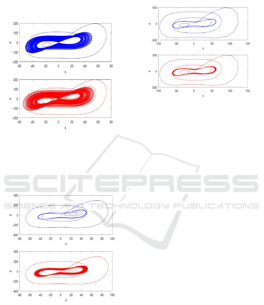
Then consider a different state of the system at
13r =
and look at the effect of noise, but in three-
dimensional space.
Figure 5:
13, 4rc==
.
As be seen from the graph, with less
r
perturbed
systems also demonstrate similar behavior. Under
these conditions, the change of attractor occurs much
earlier than in a classic system. As stochastic intensity
increases, the stochastic analogue of the Lorenz
attractor with substantially smaller
r
can be
observed. Overall, there is a negative relationship
between the stochastic factor
c
and the bifurcation
values of
r
. It is interesting to see how the system
works with large values of
r
. We start with
200r =
ISAIC 2022 - International Symposium on Automation, Information and Computing
72

and build a determine system (blue color with
0c =
)
and interfered system (red color with
5c =
).
Figure 6:
200, 0, 5rcc===
.
The graphs are quite similar, and here we clearly
see auto-oscillating mode. By increasing
r
to 300
(Figure 7), and then up to 500 (Figure 8), we can
obtain a predictable result, based on fact that
r
is an
analogue of the Rayleigh number.
Figure 7:
300, 0, 5rcc===
.
As parameter
r
increases, the role of noise will
gradually decrease. The system will be a stochastic
analogue of the auto-oscillating movement, which
will differ from the unperturbed system only by a
slight irregularity of the trajectory.
Figure 8:
500, 0, 5rcc===
.
5 CONCLUSIONS
In conclusion we would like to make the following
observations and draw a parallel with the real
physical system. All in all, it seems quite logical that
stochastic interferences strengthen quasi-stochastic
oscillations around equilibrium positions. As a result,
a trajectory similar enough to the Lorenz strange
attractor appears at smaller
r
. The same changes can
be observed, for example, in real physical systems,
where turbulence occurs earlier in the presence of
some noise source than without it. Then, gradually,
the noise reduces effect on the system, because the
Rayleigh number is already high enough. The
behavior of the system after the noise appearance
demonstrates quite clearly that stochastic interference
plays a significant role in describing turbulence.
Lorenz wanted to use his model for long-term
weather forecasting (Lorenz, 1963). Moreover, he
wanted to prove the theoretical existence of such a
method. By and large, due to the significant impact of
additive interference, it is unlikely that such a method
will ever be developed.
REFERENCES
Danilov Yu.A. Lectures on Nonlinear Dynamics: An
Elementary Introduction. 2017. Publ. by URSS.
Moscow. 208 P. (in Russian).
Isaev R.R., Maltseva A.V., Tikhomirov V.V. and Nefedov
V.V. Stability of the Lorenz system // Proc. of the
Int. Sci. Conf. “Actual problemsof applied
mathematics, informatics and mechanics”. Russia.
2022. P.P. 90-98. (in Russian)
http://www.amm.vsu.ru/conf/archivs_downloadАППМИ
М-2021.pdf
Numerical Study of Stochastic Disturbances on the Behavior of Solutions of Lorenz System
73

Kloeden P.E. and Platen E. Numerical Solution of
Stochastic Differential Equations. 1995. Springer. 636
P.
Kulchitski O.Yu., Kuznetsov D.F. Numerical simulation of
stochastic systems of linear stationary differential
equations. Differential Equations and Control
Processes (e-journal of S.-Petersburg State University).
1998. No. 1. P. 41-65. (in Russian).
https://diffjournal.spbu.ru/EN/numbers/1998.1/issue.ht
ml
Kuznetsov D.F. Stochastic differential equations: theory
and numerical solution practice. S.-Petersburg.
Printed by Politechnical University (Russia). 2010.
816 P. (in Russian).
Leonov G.A., Kuznetsov N.V. On differences and
similarities in the analysis of Lorenz, Chen, and Lu
systems (PDF). Applied Mathematics and
Computation. 2015. Vol. 256. P.P. 334–343
doi:10.1016/j.amc.2014.12.132
Lorenz E.N. Deterministic Nonperiodic Flow. J. Atm. Sci.
1963. V.20, P. 130-141.
Rozanov Yu.A. Probability Theory, Random Processes and
Mathematical Statistics. 2012. Springer. 259 P.
Sparrow C. The Lorenz equations: Bifurcations, chaos and
strangeattractors. 1982. Springer-Verlag. New York.
269 P.
ISAIC 2022 - International Symposium on Automation, Information and Computing
74