Implementation of Particle Swarm Optimization (PSO) Method in
Minimum Quantity Lubrication (MQL) Optimization to Obtain
Optimal Machining in CNC Milling Machine
Yogi Muldani Hendrawan, Faza Husnan Anshori, Andri Pratama, Herman Budi Harja, Pandoe
and Akil Priyamanggala Danadibrata
Department of Manufacturing Engineering, Manufacturing Polytechnic Bandung, Jalan Kanayakan No. 21, Dago,
Coblong, Bandung, 40135, Indonesia
Keywords: Minimum Quantity Lubricant, Particle Swarm Optimization, CNC Milling Machine, ISO 14001, Regression.
Abstract: One of the machining processes used is the milling process with CNC milling machines equipped with cutting
fluid to reduce the impact of the cutting process. One of the techniques of cutting fluid is to use MQL
(Minimum Quantity Lubricant) as an application of ISO 140001 in reducing coolant waste in the environment
which has the advantage of being more economical in reducing friction between the tool and the workpiece,
thereby reducing the temperature rate in the cutting tool. The CNC tool machine of Politeknik Manufaktur
Bandung is equipped with MQL (Minimum Quantity Lubricant) with Arduino control which has no
parameters for optimum coolant discharge during the machining process.
In this study, the Particle Swarm Optimization (PSO) method was used, which is one of the optimization
methods for making decisions used in the manufacturing process by looking for a minimum value. There
sulting from the milling process becomes a response in the process on CNC milling machines to obtain the
characteristics of an effective discharged lubricant discharge. Some parameters such as cutting depth and
feeding speed for aluminum and steel materials St37 were identified as experimental data for response. The
data was searched for equations with regression, so in this study a polynomial regression model was chosen
that could describe the data value better than linear regression.
Polynomial equations are calculated with the Particle Swarm Optimization (PSO) algorithm to find the
optimum flowrate. So that the minimum discharge obtained on aluminum material for a feeding depth of less
than 0.85 mm is 25ml/h, and more than 0.85mm is 85ml/h. while for St.37 material the feeding depth of less
than 0.35 mm is 25ml/h, and more than 0.35mm is 85ml/h.
1 INTRODUCTION
One of the machine tools that uses automation
systems that are commonly used by industry today is
CNC (Computer Numerical Control) machines. In the
machining process, it cannot be separated from the
use of coolant or coolant to clean and cool the
workpiece and cutting tools. Related to
environmental issues regulated in ISO 140001 on
recommendations for reducing coolant waste in the
machining process. Therefore, a method is needed by
using a coolant that is as minimal as possible with
more environmentally friendly materials. One of the
methods used is minimum quantity lubricant (MQL).
Related to environmental issues regulated in ISO
140001 on recommendations for reducing coolant
waste in the machining process. Therefore, a method
is needed by using a coolant that is as minimal as
possible with more environmentally friendly
materials. One of the methods used is minimum
quantity lubricant (MQL).
Be advised The development of POLMAN CNC
machine tools already has a cooling system by
installing a minimum quantity lubricant (MQL)
method cooling system with Arduino control on a
MINI CNC Milling machine made by POLMAN.
However, the Minimum Quantity Lubricant (MQL)
does not yet have an optimum discharge. The Particle
Swarm Optimization (PSO) method is used as one of
the optimization algorithms that can solve complex
optimization problems if solved in an exact manner.
Hendrawan, Y., Anshori, F., Pratama, A., Harja, H., Pandoe, . and Danadibrata, A.
Implementation of Particle Swarm Optimization (PSO) Method in Minimum Quantity Lubrication (MQL) Optimization to Obtain Optimal Machining in CNC Milling Machine.
DOI: 10.5220/0011891500003575
In Proceedings of the 5th International Conference on Applied Science and Technology on Engineering Science (iCAST-ES 2022), pages 821-827
ISBN: 978-989-758-619-4; ISSN: 2975-8246
Copyright © 2023 by SCITEPRESS – Science and Technology Publications, Lda. Under CC license (CC BY-NC-ND 4.0)
821

2 THEORY AND RESEARCH
METHODS
The machining process is the process of removing
material parts (removal of material) with the help of
cutting tools on the machine. The machining process
aims to achieve the desired. geometry, size, surface
smoothness, and function of the workpiece in the
process.
The principle of the machining process is that the
part of the workpiece that is not needed will be
removed by means of a cutting process using a cutting
tool with a rotating or shifting motion. Here are the
five elements of the machining process, namely
(Rochim, 1993):
1) cutting speed: v (m/min);
2) feeding speed: vf (mm/min);
3) depth of cut: 𝑎 (mm);
4) cutting time: tc (min);
5) rate of metal removal: z (cm3 /min);
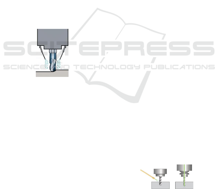
2.1 Wet Machining
Figure 1: Wet machining.
Wet machining method is the use of coolant in the
machining process aimed at cooling the cutting tool
used. According to how coolant is given to the Wet
Machining method, it can be divided into three types
of cooling processes, namely: flooded to the
workpiece (Flood application), sprayed (Jet
application fluid) and atomized (Mist application
fluid).
The use of this many coolants in the machining
process can accelerate the rate of cooling that occurs.
With the material studied is the steel type AISI 422
states that, for wet engine temperatures are in the
range of 26-30 °C, which is the temperature spreading
throughout the cutting surface with pressure from the
engine pump, and absorbing the temperature from the
tool, workpiece and furious (Glanis, 2008). In this
study, synthetic fluids were used, synthetic fluids
consisted of a mixture of organic and inorganic
alkaline materials and added with additives to ward
off corrosion. This liquid has the best cooling
capacity when compared to other coolants.
2.1.1 Minimum Quantity Lubrication
Minimum quantity lubrication (MQL), using a very
small amount of liquid for the machinery process in
the form of an aerosol formed from a mixture of
coolant and air using a venturi working insert. The
pressure difference between the air pressure channel
in and output through the nozzle is lower pressed so
that the coolant enters the mist lubrication spray
system.
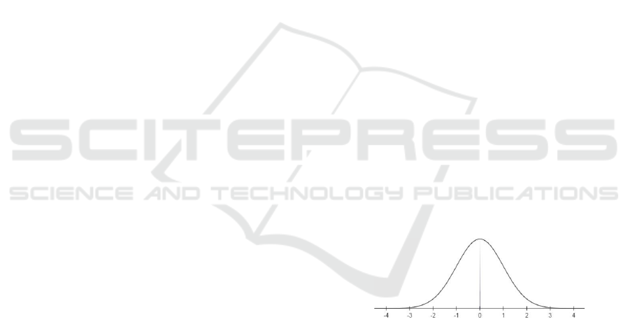
MQL has two types of coolant supply, namely
External MQL Supply and Internal MQL Supply. The
application of MQL although the provision of a
minimum coolant but is able to produce better tool
life, better surface finish, better furious shape,
reduced cutting power and on the workpiece, cutting
tools and parts affected by the coolant will provide
resistance to oxidation, providing environmental
friendliness
Minimum quantity lubrication (MQL) is a total-
loss lubrication method, which means using new and
clean lubricants only one-time use. But as a general
rule, 25-85 ml / hour on a cutting tool less than 40 mm
in diameter,
2.2 Particle Swarm Optimization
(PSO)
The PSO algorithm was invented by Kennedy and
Eberhart in 1995, mimicking the behavior of a flock
of seagulls that fly together to forage or nest. Pso
algorithms can easily reach global and optimal points
because of their ease of application to solve problems
and have consistent performance, so that PSO
algorithms are good and effective for solving
optimization problems.
The PSO algorithm, birds are represented as
"particles", where each particle represents a possible
solution to an optimization problem. The word
"particle" denotes an individual, where each
individual is connected using their own intelligence
(Intellegence) and influences the behavior of their
group. Thus, if one of the particles finds the fastest
Figure 2: Minimum quantity lubrication type.
iCAST-ES 2022 - International Conference on Applied Science and Technology on Engineering Science
822

and right path to the food source then the rest of the
other group can immediately follow the path even
though the location of the member is far from the
group.
2.2.1 PSO Algorithm Structure
There are several components in the PSO Algorithm
including the following:
1. Swarm, which is the number of particles in
a population in an algorithm. The size of the
swarm depends on how complex the
problem is. In general, the swarm size in
PSO algorithms tends to be smaller
2. Particle, is an individual in a swarm that
represents the solution of solving a
problem. Each particle has a position and
speed determined by the representation of
the solution at that moment.
3. Personal best (pbest), is the best position
that a particle has ever achieved by
comparing fitness in the current particle
position with before. Personal best is
prepared to get the best solution.
4. Global Best (gbest), is the best position of
particles obtained by comparing the best
fitness values of all particles in the swarm.
5. Velocity (velocity), v is a vector that
determines the direction of displacement of
the particle's position. Velocity changes are
made each iteration with the aim of
correcting the original particle position.
6. Inertial weight (inertia weight), w is used to
control the impact of the velocity change
given by the particle.
7. Acceleration coefficient, is the controlling
factor of the extent to which particles move
in one iteration. In general, the values of the
acceleration coefficients c1 and c2 are the
same, namely in the range of 0 to 4.
Nevertheless, the value can be determined
by yourself for each different study
2.3 Mathematical Equations with
Regression
The term regression according to statisticians applied
to almost all areas of science, to estimate or foresee
the value of one variable based on another variable
whose value has been known, and both variables have
a functional or causal relationship with one another.
Before creating a regression equation it is necessary
to determine the form of the data distribution. So it is
better to make it in a scatter diagram or scatter
diagram and then look at the regression equation that
is closest based on the number of data distribution so
that the deviation that occurs can be as small as
possible.
There are two types of regression sought in this
study:
Multiple linear regression equation
𝑌̂ = 𝑏0 + 𝑏1 𝑋1 + 𝑏2 𝑋2
(1)
Ý = function value (bound variable)
b0 = constant value
b1 = partial regression coefficient of X1 b2 = coefisen
partial regression of X2
Polynomial regression equation
𝑌 = 𝑎 + 𝑏𝑋 + 𝑐𝑋2 (2)
Y = function value (bound variable) a = constant
value
b = the value of the coefficient constant X c =
coefficient constant value X2
X = free variable value
In this study the search for regression equations was
carried out with the help of matlab software and IBM
SPSS.
2.3.1 Normality Test
Parametric statistical analysis is an analysis used to
test population parameters through statistical analysis
or test population size through sample data. In order
for the data to be tested for parametric analysis, it is
required that the data must be normally distributed
(Widana,2020).
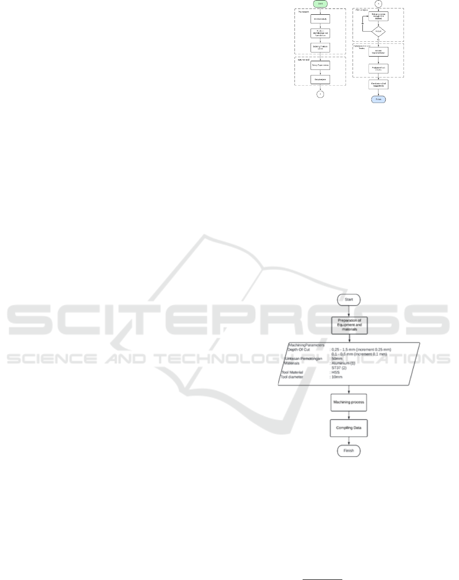
Figure 3: Normal distribution chart.
A data will form a normal distribution curve with
the shape of the bottom open curve or resemble a bell
with two parameters, namely average and standard
deviation. The shape of the normal distribution curve
can be seen in the figure below:
Normality tests can also be performed by plotting
probability plots. Where a data in the regression
model is said to be normal if the plotting data (dots)
depicting the actual data follows a diagonal line
(Widana,2020).
Implementation of Particle Swarm Optimization (PSO) Method in Minimum Quantity Lubrication (MQL) Optimization to Obtain Optimal
Machining in CNC Milling Machine
823

2.3.2 T Test (Partial)
Partial tests are used to show how much influence an
independent variable or free variable has on a
dependent variable or bound variable.
Step-by-step in performing partial testing on data
(Nuryadi, 2017):
1. Determine the significance value of the α (the value
used α = 0.05).
2. Looking for the calculated value of t
3. Comparing the calculated t value with t table (α/2
; n-k-1)
If:
Sig value. > α significantly different (no relationship)
Sig value. < α does not differ significantly (there is a
relationship)
t count < t the table differs significantly (there is no
relationship)
t count > t the table does not differ significantly
(there is a relationship)
2.3.3 F Test (ANOVA)
The F test or Analysis Of Variance (ANOVA) is one
of the tests in test statistics used to test the distribution
or variance means in variables simultaneously or
together (Nuryadi, 2017).
Steps in conducting the F Test used (Nuryadi, 2017):
1 Specifies the significance value of the α (the
value used α = 0.05).
2 Looking for the calculated F value.
3 Comparing F count with F Table (k ; n-k) If:
Sig value. > α significantly different (no relationship)
Sig value. < α does not differ significantly (there is a
relationship)
F count < F the table differs significantly (there is no
relationship)
F count > F the table does not differ significantly
(there is a relationship)
2.4 Research Methods
In this study, an experimental method was used,
namely a method by testing the Minimum Quantity
Lubricant (MQL) with quality controlled based on
predetermined parameters. These parameters are
Depth of Cut (DoC), the composition of the lubricant
flowrate, RPM and feeding that have been
determined.
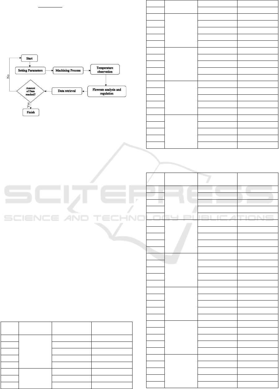
Figure 4: Research method flow chart.
2.4.1 Activity Flowchart
Flowchart planning activities optimization minimum
quantity lubricant on CNC machines, consisting of
pre-research activities, data retrieval, PSO analysis,
and implementation and testing.
2.4.2 Experiment Strategy
Strategic planning in conducting minimum quantity
lubricant (MQL) optimization experiments in
accordance with the selected parameters. The
activities on the experimental strategy can be seen in
the flow chart below:
Figure 5: Experiment strategy flow chart.
2.4.3 Machining Parameters
Here is the determination of the parameters for
aluminum and St.37 materials:
1. Aluminium
Vc aluminium = 80 m/mnt
Feed per teeth= 0.02
𝑅𝑝𝑚 =
1000 𝑥 80
𝜋 𝑥 10
= 2546.47 ≈ 2500 rpm
𝑓𝑒𝑒𝑑𝑖𝑛𝑔(𝑠) = 2500 × 0.02 × 4 = 200 𝑚𝑚/𝑚𝑖𝑛
2. St.37
Vc St.37= 20 m/mnt
Feed per teeth = 0.02
iCAST-ES 2022 - International Conference on Applied Science and Technology on Engineering Science
824

𝑅𝑝𝑚 =
1000 𝑥 20
𝜋 𝑥 10
= 636.61 ≈ 650 rpm
𝑓𝑒𝑒𝑑𝑖𝑛𝑔(𝑠) = 650 × 0.02 × 4 = 52 𝑚𝑚/𝑚𝑖𝑛
To obtain the data is carried out machining process
with predetermined parameters. The following is a
flow chart of the process of machining activities for
data collection:
Figure 6: Machining experiment flow chart.
The optimization process is carried out with the
model of mathematical equations obtained so that the
optimum value of the flow rate of the corresponding
machining process is obtained. The Optimization
process is carried out according to the flow chart of
the algorithm starting from the initialization of the
position, the initial speed, the maximum iteration.
then, calculate the value of each particle through the
value of the function to determine the initial Pbest and
Gbest. after that, do an update of position and speed.
recalculates the fusion value based on the new
position up to the specified iteration limit, and then
sorted to find the minimum solution.
3 RESULT
3.1 Research Methods
The data taken is the influence into the feeding and
flowrate on the temperature response that occurs
during the machining process. So that data for
aluminum and St.37 were obtained as follows:
Table 1: Alumunium experiment result, n=2500 rpm,
feeding=200 mm/min.
No
DoC [mm]
Flow Rate
[ml/h]
Temperature
[
o
C]
1
0.25
25
24.9
2
40
24.9
3
55
24.3
4
70
24.5
5
85
26.4
6
0.5
25
26.9
7
40
27
8
55
27.2
9
70
27.4
10
85
27.4
11
0.75
25
28.4
12
40
28.8
13
55
28.4
14
70
28.5
15
85
28.1
16
1
25
29.2
17
40
28.8
18
55
30
19
70
29.8
20
85
28.9
21
1.25
25
31.1
22
40
31.6
23
55
32.4
24
70
32.4
25
85
31.8
26
1.5
25
33.3
27
40
33.1
28
55
32.9
29
70
32.1
30
85
30.1
Table 2: ST37 experiment result, n = 650 rpm, feeding = 32
mm/min.
No
DoC [mm]
Flow Rate
[ml/h]
Temperature
[
o
C]
1
0.1
25
25.8
2
40
26.5
3
55
26.2
4
70
26.1
5
85
26.4
6
0.2
25
27.1
7
40
27.1
8
55
27.7
9
70
27.7
10
85
27.4
11
0.3
25
28.1
12
40
28.3
13
55
28.1
14
70
27.9
15
85
27.8
16
0.4
25
28.3
17
40
28.2
18
55
28.3
19
70
28.2
20
85
28.2
21
0.5
25
29
22
40
29.1
23
55
29.2
24
70
28.5
25
85
28.6
26
0.6
25
28.9
27
40
29
28
55
28.8
29
70
29.1
30
85
28.9
Implementation of Particle Swarm Optimization (PSO) Method in Minimum Quantity Lubrication (MQL) Optimization to Obtain Optimal
Machining in CNC Milling Machine
825

3.2 Regression Equation Results from
Experiments
The linear regression equations from the experiment
obtained using IBS SPSS is:
𝑌1 = 23,98 − 0,002 𝑋1 + 5,879 𝑋2
𝑌2 = 26,147 − 0,001 𝑋1 + 5,240 𝑋2
The polynomial regression equations from the
experiment obtained using Matlab is:
𝑌1 = 21,42 + (0,06564 × 𝑥1) + (7,819 × 𝑥2)
− (0,0003333 × 𝑥12)
− (0,03528 × 𝑥1 × 𝑥2)
𝑌2 = 24,81 + (0,006444 × 𝑥1) + (13,47 × 𝑥2)
− (0,02 × 𝑥1 × 𝑥2) − (10.18 × 𝑥22)
Information:
Y1 = Suhu Aluminium Y2 = Suhu St.37
x1 = Flowrate
x2 = Depth of Cut
3.3 Comparison of Linear Regression
Equations and Polynomials
To see the regression equation that is suitable for
processing with PSO, the role of regression equation
is carried out
Table 3: Comparison of the coefficient of determination of
aluminum regression.
Multiple Linear Regression
Polynomial Regression
0,916
0,9327
Table 4: Comparison of aluminum regression errors.
Multiple Linear
Regression
Polynomial
Regression
0,577942
0,501499
Table 5: Comparison of regression coefficients of
determination St.37.
Multiple Linear
Regression
Polynomial
Regression
0,865
0.9404
Table 6: Comparison of St.37 regression errors.
Multiple Linear
Regression
Polynomial Regression
0,288933
0,202568
3.4 PSO Algorithm Calculation Results
Here are the results of the pso algorithm optimization
calculation through Matlab software:
Table 7: Alumunium PSO algorithm results.
No
DoC
[mm]
PSO Flow Rate
Results [ml/h]
Best Fitness PSO
Results [
o
C]
1
0.05
25
23.1995
2
0.1
25
23.5464
3
0.15
25
23.8932
4
0.2
25
24.2401
5
0.25
25
24.5869
6
0.3
25
24.9338
7
0.35
25
25.2806
8
0.4
25
25.6275
9
0.45
25
25.9743
10
0.5
25
26.3212
11
0.55
25
26.668
12
0.6
25
27.0149
13
0.65
25
27.3617
14
07
25
27.7086
15
0.75
25
28.0554
16
0.8
25
28.4023
17
0.85
85
28.6885
18
0.9
85
28.9295
19
0.95
85
29.1705
20
1
85
29.4115
21
1.05
85
29.6525
22
1.1
85
29.8935
23
1.15
85
30.1345
24
1.2
85
30.3755
25
1.25
85
30.6166
26
1.3
85
30.8576
27
1.35
85
31.0986
28
1.4
85
31.3396
29
1.45
85
31.5806
30
1.5
85
31.8216
Table 8: Alumunium PSO algorithm results.
No
DoC [mm]
PSO Flow Rate
Results [ml/h]
Best Fitness PSO
Results [
o
C]
1
0.05
25
25.5942
2
0.1
25
26.1663
3
0.15
25
26.6875
4
0.2
25
27.1579
5
0.25
25
27.5773
6
0.3
25
27.9459
7
0.35
85
28.2302
8
0.4
85
28.4369
9
0.45
85
28.5928
10
0.5
85
28.6977
11
0.55
85
28.7518
12
0.6
85
28.7549
13
0.65
85
28.7072
14
07
85
28.6085
15
0.75
85
28.4590
iCAST-ES 2022 - International Conference on Applied Science and Technology on Engineering Science
826

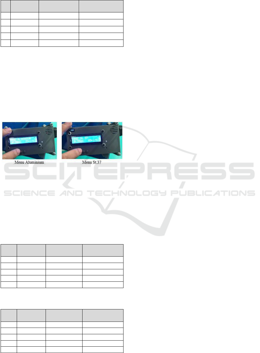
Table 8: Alumunium PSO algorithm results (cont.).
No
DoC [mm]
PSO Flow Rate
Results [ml/h]
Best Fitness PSO
Results [
o
C]
16
0.8
85
28.2585
17
0.85
85
28.0072
18
0.9
85
27.7049
19
0.95
85
27.2728
20
1
85
26.9477
3.5 Implementation on Arduino
Implementation of optimization results in the form of
a data base on the Arduino from the optimum flowrate
results for feeding recommendations. The add-on
program to MQL is a new menu for recommendations
of MQL optimum values. Flowrate recommendation
menu display:
Table 9: Arduino menu display.
3.6 Results Test and Validation Results
The test results are carried out to validate the results
of the optimization data calculated using the PSO
method, by testing the feeding in accordance with the
optimum flowrate obtained. here are the results of
MQL testing with optimization results with Particle
Swarm Optimization.
Table 10: Validation of optimum flowrate comparison
(Alumunium).
DoC
Temp
with MQL
Temp without
MQL
PSO Measure.
Temp.
0.15
24.8
25.8
23.89
0.25
25.9
26.4
24.58
0.35
26.3
26.8
25.28
0.5
27.2
28.1
26.32
0.85
28.8
30.8
28.68
Table 11: Validation of optimum flowrate comparison
(ST37).
DoC
Temp
with MQL
Temp without
MQL
PSO Measure.
Temp.
0.2
27.8
30.9
27.17
0.25
28.5
31.5
27.57
0.3
28.9
31.9
27.94
0.35
29.3
32.7
28.23
0.4
29.8
33.2
28.43
4 CONCLUSIONS
To obtain the optimal lubricant discharge in MQL,
data collection is carried out with depth of cut and
flowrate parameters. so that the results of the data will
be processed to obtain the regression equation. The
Regression Equation will be calculated through the
PSO algorithm and the results will be obtained:
In aluminum materials the discharge of lubricant
for a depth of less than 0.85mm is 25 ml/h.
Meanwhile, more than 0.85 ml/h is 85 ml/h.
In St.37 materials the discharge of lubricant for
depths of less than 0.35mm is 25 ml/h. Meanwhile,
more than 0.35 ml/h is 85 ml/h.
REFERENCES
Cholissodin, I. Swarm Intellegence (Teori & Case Study).
Malang: Fakultas Ilmu Komputer Universitar
Brawijaya, 2016.
Dhanasaputra, N., & Santosa, B. Pengembangan algoritma
cat swarm optimization. Jurnal ITS, pp 3, 2010.
Erny. "Optimasi Pola Penyusunan Barang Dalam Peti
Kemas Menggunakan Algoritma Particle Swarm
Optimization," Skripsi,. Makasar: Universitas
Hassanudin, 2013.
Glanis, N. I., Manolakos, D. E., & Vaxevanidis, N. M. .
Comparison Between Dry and Wet Machining of
Stainles steel. Proceedings of the 3rd International
Conference on Manufacturing Engineering (ICMEN),
91-98, 2008.
Ihsyani, T. A. "Pembuatan Sistem Minimum Quantity
Lubrication (Mql) Dengan Kontrol Arduino Pada Mesin
CNC." Tugas Akhir Diploma, Bandung: Jurusan Teknik
Manufaktur Politeknik Manufaktur Bandung, 2021.
Nuryadi, Astuti, T. D., Utami, E. S., Budiantara, M. "Dasar-
dasar statistic penelitian .", Yogyakarta: SIBUKU
MEDIA, 2017.
Rochim, T. "Teori dan teknologi Permesinan .", Bandung: ITB
Press, 1993.
Widana, W, Muliani, P. L. "Uji persyaratan analisis .",
Lumajang: KLIK MEDIA, 2020.
Implementation of Particle Swarm Optimization (PSO) Method in Minimum Quantity Lubrication (MQL) Optimization to Obtain Optimal
Machining in CNC Milling Machine
827