Research on Competitiveness Model of the Global Energy and
Power Interconnection
Jie Yang
*
and Jun Liu
State Grid Energy Research Institute Co., Ltd, Beijing, 102209, China
Keywords: Competitiveness Model, Global Energy and Power Interconnection, Fuzzy-Logarithmic, Anti-Entropy.
Abstract:
The global energy and power interconnection has great significance in achieving optimal allocation of
global energy resources. To quantify the demand of long-distance transmissions in various areas, this paper
proposes an assessing model for the competitiveness model of the global energy and power interconnection.
This quantified model is established from the physical and mathematical levels, to fully reflect the
complexity and difficulty of energy and power interconnection system, a new combination weighting
approach consists both of fuzzy-logarithmic and anti-entropy methods is adopted, meanwhile fuzzy
membership concept is introduced into overall evaluation for Belt and Road energy and power
interconnection.
1 INTRODUCTION
In order to alleviate the crisis of global energy
resources, and eliminate the environmental pollution
caused by fossil energy consumption, China has
promoted the construction of global energy and
power interconnection (Liu, 2016; Guan, 2016; Xia,
2016). Current practices in global energy and power
interconnection are still in the start-up step, lack of
systematic methods and tools for quantitative
assessment. In terms of research considerations,
most of the existing studies do not have sufficient
depth of comprehensive analysis of influencing
factors, focusing on the simple synthesis of energy
and power resource conditions and project economy,
lack of consideration of important factors such as
economic and environment (Karunanithi, 2017;
Kim, 2016; Wei, 2016). In terms of research
methods, the existing research is based on a simple
and intuitive subjective evaluation system, which
makes it difficult to fully reflect the complexity of
the energy and power system (Xing, 2017; Liang,
2018). Therefore, establishing a scientific and
reasonable quantitative model and assessing system
for the competitiveness of the global energy and
power interconnection, will provide decision-
making reference for the construction of energy and
power interconnection in the Belt and Road.
2 ASSESSING MODEL FOR THE
COMPETITIVENESS OF
ENERGY AND POWER
INTERCONNECTION
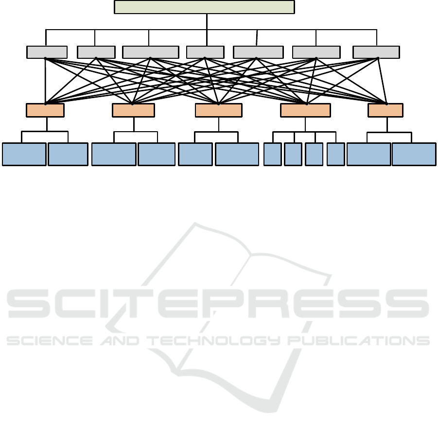
2.1 Physical Model
In the physical model, the factors influencing the
development of energy and electric power are
classified and sorted, and the key influencing factors
of optimal competitiveness of energy and power
interconnection are extracted from the target layer,
object layer, control layer and index layer. The
target layer describes the main tasks of the assessing
model. The object layer consists of research objects,
including renewable energy generation
(hydropower, wind power, solar energy and other
power generation) and non-renewable energy (coal,
gas, nuclear, oil and electricity). A total of 12
assessing factors are selected. These factors are
summarized into multiple subsystems, defined as
control layers, each of which directly affects the
evaluation of the object layer. At the bottom is the
indicator layer, which sets specific indicators
according to the different evaluation objectives of
the corresponding subsystems, and are the basis for
quantitative and comprehensive assessment, as
shown in Figure 1.
Yang, J. and Liu, J.
Research on Competitiveness Model of the Global Energy and Power Interconnection.
DOI: 10.5220/0011735000003607
In Proceedings of the 1st International Conference on Public Management, Digital Economy and Internet Technology (ICPDI 2022), pages 285-291
ISBN: 978-989-758-620-0
Copyright
c
 2023 by SCITEPRESS – Science and Technology Publications, Lda. Under CC license (CC BY-NC-ND 4.0)
285

A1: Optimal competitiveness of energy and power interconnection
C1:Resource C2:Economy C3:Technique C4:Environment C5:Policy
B1:Coal B2:Gas B3:Nuclear B4:Oil B5:Hydro B6:Wind B7:Solar
D1:Developing
potentiality
D2:Contrary
distribution
D3:Production
cost
D4:External
cost
D5:Energy
conversion
D6:supporting
capacity
D7:
CO
2
D8:
SO
2
D9:
N
x O x
D10:
Dust
D11:Policy
support
D12:Policy
execute
Figure 1: Physical model for the competitiveness of energy and power interconnection.
2.1.1 Resource Subsystem
In order to effectively describe the influence of
resource subsystems on competitiveness of energy
and power interconnection, the developing
potentiality (D1) and contrary distribution (D2) are
selected as the evaluation indicators under the
resource subsystem. Among them, the contrary
distribution refers to the distance of energy
resources and load center of power generation in the
regional power grid.
2.1.2 Economy Subsystem
The pursuit of economy is one of the important
goals of allocation energy and power
interconnection in regional power grid, and
economic subsystem (C2) is mainly to depict the
influence of economic factors on the power supply
structure of regional power grid. The indicators
reflecting the energy economy of power generation
include investment cost, fuel cost, operation and
maintenance cost and environmental cost, and this
paper finally refines the production cost (D3) and
external cost (D4) as the evaluation indicators under
the economic subsystem.
2.1.3 Technique Subsystem
In this paper, the energy conversion (D5) and
support capacity (D6) are set as the specific
indicators of the technique subsystem (C3). The
level of energy conversion is a quantitative index,
characterizing the efficiency of various types of
power generation technology applications, and
different energy efficiency varies according to
equipment level and technology level. The support
capacity takes into account the average utilization
coefficient of power supply, peak adjustment
capacity and power generation efficiency.
2.1.4 Environment Subsystem
To depict the environmental impact of various
power supplies, this section selects carbon dioxide
emissions (D7), sulfur dioxide emissions (D8),
nitrogen oxide emissions (D9) and dust emissions
(D10) as four specific indicators under the
environmental subsystems.
2.1.5 Policy Subsystem
This paper uses a policy subsystem (C5) to describe
the impact of energy policies on the development of
regional grid power supplies. In studying the impact
of policy subsystems on power supply development,
we need to consider not only the formulation
(output) of energy policy, but also the effectiveness
(feedback) of energy policy. Based on this, this
paper uses policy support (D11) and policy execute
(D12) to describe the impact of policy subsystems.
2.2 Mathematical Model
In the previous section, a physical model for the
competitiveness of energy and power
interconnection was established from five
subsystems: resources, economy, technique,
environment and policy. The content of this section
is to quantify the above-mentioned physical model
indicators one by one, and then build a mathematical
model for the competitiveness of energy and power
interconnection.
ICPDI 2022 - International Conference on Public Management, Digital Economy and Internet Technology
286

2.2.1 Indicator Layer Calculation
• Index Assignment
The first step in the calculation of the indicator layer
is to assign 12 energy and power indicators,
according to the nature characteristics of each
indicator, this section adopts two indicator
assignment methods: 1) for quantitative energy and
power indicators, this paper studies literature reports
issued by the authorities (including The
International Energy Agency, the U.S. Energy
Information Administration, BP, and Bloomberg
New Energy Finance, etc.) to obtain important data
information; 2) for qualitative energy and power
indicators, this paper designs the indicator scoring
table, which is assigned by a number of energy and
power industry experience experts. Then we can get
the assignment matrix B
k
of the nth indicators of the
kth control layer subsystem where B
k
=[b
1
, b
2
,…, b
n
].
• Normalization
The second step of the calculation of the indicator
layer is normalization processing: each energy and
power indicator has different physical significance
and value range, in order to enable it to carry out
comprehensive analysis, it is necessary to normalize
so that the energy and power indicators have a
consistent effect on the power evaluation effect.
Then we can get the normalization matrix Z
k
of the
nth indicators of the kth control layer subsystem
where Z
k
=[z
1
, z
2
,…, z
n
].
• The selection of the Fuzzy Membership
function
The third step is to evaluate each indicator, the
rating is excellent, good, medium and poor, and
comment set can be expressed as P={p
1
, p
2
, p
3
, p
4
}.
For the normalization matrix Z
k
, the Fuzzy
demarcation interval of 4 state levels is given, and
the membership function of each state level is
established.
()
1
0 0.6
0.5 5 0.7 0.6< 0.8
1 0.8
p
z
lz z
z
≤


=+− ≤


>

(1)
()
()
2
0 0.4
0.5 5 0.5 0.4< 0.6
0.5 5 0.7 0.6< 0.8
0 0.8
p
z
zz
l
zz
z
≤


+− ≤

=

−− ≤


>

(2)
()
()
3
0 0.2
0.5 5 0.3 0.2< 0.4
0.5 5 0.5 0.4< 0.6
0 0.6
p
z
zz
l
zz
z
≤


+− ≤

=

−− ≤


>

(3)
()
4
1 0.2
0.5 5 0.3 0.2< 0.4
1 0.4
p
z
lz z
z
≤


=+− ≤


>

(4)
2.2.2 Combination Weighting
Because of the ambiguity of the assessment
indicators, this paper uses fuzzy logarithmic method
to weighting the indicators. The fuzzy judgment
matrix
A

is shown in formula (5), which represents
the relative importance of the factor D
i
comparison
with factor D
j
, l
ij
and m
ij
represent the lower and
upper bounds of the triangular fuzzy
ij
a

, and u
ij
represents the optimal value.
()
() ( ) ()
()() ()
()( )
()
11 12 1 12 12 12 1 1 1
21 22 2
21 21 21 2 2 2
12
111 2 22
1, 1,1 , , , ,
,, 1,1,1 ,,
,, ,, 1,1,1
nnnn
n
nnn
ij
nn
nn nn
nnn n nn
aa a lmu lmu
aa a
lmu lmu
Aa
aa a lmu lmu
×






== =







 

 




    
 

(5)
Set as the weight of the indicator D
i
, the
logarithmic form of the fuzzy judgment matrix is as
follows:
ln ln
ln
ln ln
ln
ln ln
ln
ln ln
i
ij
j
i
ij
ij ij j
i
ij
j
i
ij
j
i
ij
ij ij j
w
l
w
w
m
ml w
w
w
w
u
w
w
m
um w
μ


′
−



′

′


≤



′
−


′

=




′

′



−



′

′


>



′
−


(6)
where
()
()
ln /
ij i j
ww μ
′′
represents the membership
()
ln /
ij
ww
′′
of the fuzzy matrix
ln
ij
a

. Making
ϕ
the minimum membership,
ij
δ
and
ij
η
as non-
negative error parameters, and M as the specified
large values, the fuzzy logarithmic model can be
expressed as:
i
w
′
Research on Competitiveness Model of the Global Energy and Power Interconnection
287

()
()
()
()
1
2
22
11
min 1
ln / ln
ln / ln
..
,0
,0
nn
ij ij
iji
i j ij ij ij ij
i j ij ij ij ij
i
ij ij
JM
xx ml l
x
xum u
st
x
ϕδη
ϕδ
ϕη
λ
δη
−
==+
=− + × +

−− +≥


−+ − + ≥−


≥


≥



(7)
where . According to the inequality, we
can find the optimization solution , and then get
the weight value of the fuzzy judgment matrix:
()
()
*
*
1
exp
i
i
n
i
j
x
w
x
=
′
=

(8)
Although fuzzy logarithmic method solves the
problem of the complex system of energy and power
supply, it still belongs to the subjective weighting
method, so the anti-entropy method is added to
amend the above method.
It should be noted that the anti-entropy method
measures the comparison between the evaluation
objects, focusing on the comprehensive evaluation
of the seven kinds of power supply in the object
layer. If z
kj
is the standard value of indicator i under
the kth evaluation object, the information output of
indicator i is anti-entropy E
i
is shown as:
()
()
7
1
ln 1
ikiki
k
E
zz
=
′′
=− ⋅ −

(9)
7
1
ki
ki
ki
k
z
z
z
=
′
=

(10)
The weight coefficients output by anti-entropy
method is:
1
/
n
ii j
j
wE E
=
′′
=

(11)
In summary, the subjective weight is
obtained by fuzzy logarithmic method, the objective
weight matrix is obtained by the anti-entropy
method, and the important coefficients and
of the main objective weights of each indicator are
calculated according to the moment estimation
theory, and the final calculation of the combined
weights is shown below.
()
()
/
/
ii ii
ii ii
www
www
α
β
′′′′

=+


′′ ′ ′′
=+


(12)
()
1
ii ii
i
n
j
jjj
j
ww
w
ww
α
β
αβ
=
′′′
+
=
′′′
+

(13)
At this point, we can get the weight vector
W
k
=[w
1
, w
2
,…, w
n
] of nth indicators of the kth
control layer subsystem.
2.2.3 Comprehensive Fuzzy Evaluation
Model
According to the membership matrix L
k
of the nth
indicators of the kth control layer subsystem and the
indicator weight vector W
k
, the membership degree
matrix G
k
of each subsystem of the control layer can
be calculated by formula (14).
() () () ()
1234kkk k k k k
GWL gp gp gp gp==


(14)
For the ith power supply, the comprehensive
evaluation membership matrix H
i
can be calculated
according to the five subsystems membership matrix
N
i
=[G
i1
, G
i2
, G
i3
, G
i4
, G
i5
], and the control layer
weight factor W
i
.
[
]
1234iii iiii
HWL h h h h==
(15)
where h
ij
(j=1, 2, 3, 4) is the membership value
corresponding to the ith power supply.
Set
λ
i
is the weight of various energy and power
supplies in the energy structure (i=1, 2, 3, 4, 5, 6, 7).
To maximize the combination of comprehensive
scoring values as the goal function, adding
resources, environment and policies and other
constraints, maximize the regional power grid power
combination of the comprehensive benefits, the
target function is as follows:
74
11
max
ijij
ij
J
qh λ
==
=⋅⋅

(16)
where q
i
is the score for membership, and q
1
=90,
q
2
=70, q
3
=50 and q
4
=30. to q4 for 90, 70, 50 and 30,
respectively. With a installed capacity of Si for the
seven energy and power supplies in the regional
grid, the optimization model needs to meet the
following constraints:
• Power demand constraints
The sum of the various energy and power
generation capacities of the regional grid must meet
the maximum forecast of regional power demand:
()
6
max
1
1
ii
i
ST D γ
=
⋅≥+

(17)
where T
i
is the utilization hours of various power
supplies, D
max
is the maximum forecast of power
demand, and
γ is the system backup rate.
• Maximum installed capacity constraints
ln
ii
x
w
′
=
*
i
x
i
w
′
i
w
′′
i
α
i
β
ICPDI 2022 - International Conference on Public Management, Digital Economy and Internet Technology
288

The installed capacity of renewable energy
should be less than the maximum economically
exploitable capacity
N
i_max
:
_maxii
SN≤
(18)
• Environmental constraints
Environmental constraints mainly consider
pollutants emitted from the atmosphere. The
emissions of sulfur dioxide, nitrogen oxides, dust
and carbon dioxide from the power supply shall be
lower than the limit of pollutant emissions:
22
6
_SO SO
1
ii i
i
ST P κ
=
⋅⋅ ≤

(19)
6
_NO NO
1
xx
ii i
i
ST P κ
=
⋅⋅ ≤

(20)
6
_YC YC
1
ii i
i
ST P κ
=
⋅⋅ ≤

(21)
22
6
_CO CO
1
ii i
i
ST P κ
=
⋅⋅ ≤

(22)
• Structure constraints
In addition, it is also necessary to consider that
the various energy and power supply weights in the
regional power grid should be between 0 and 1, and
that the sum of the weights is equal to 1.
01
i
λ ≤≤
(23)
6
1
1
i
i
λ
=
=

(24)
By solving the above-mentioned objective
function, we can get the optimal solution of weight
and installed capacity , and then the optimal
normalization score
J
*
of local power and energy for
each area can also be obtained, and the difference
between 1 and
J
*
will be the normalization score of
competitiveness for energy and power
interconnection in each area.
3 MODEL RESULTS
According to the concept of competitiveness for
energy and power interconnection and the
corresponding assessing model, the paper takes
southeast Asian power grid as an example to
analyse. Firstly, through authoritative energy
agencies to investigate the largest economic
development capacity, electricity costs and other
quantitative indicators, and according to empirical
experts to determine policy support and other
qualitative indicators, the indicator assignment
matrix B, further the indicator normalization matrix
Z is shown in Table 1.
Secondly, the fuzzy judgment matrix is
determined, and the weight value of each indicator
is obtained according to the fuzzy matrix. According
to the influence degree of each subsystem, drawing
on the authoritative research conclusions, the fuzzy
judgment matrix is set as follows:
1 1/3 1/3 1/7 1/9
31 11/31/5
31 11/31/5
73311/3
95 5 3 1
A




=




 

  


  

 



(25)
Similarly, the fuzzy judgment matrix of the
indicator layer indicator can be obtained, and use the
fuzzy-logarithmic and anti-entropy combination
weighting method proposed in this paper to get the
indicator weight matrix W, as shown in Table 2.
Table 1: Indicator normalization matrix.
Coal Gas Nuclear Oil Hydro Wind Solar
D1 0.09 0.11 0.16 0.06 0.80 0.90 1.00
D2 0.80 0.90 1.00 0.90 0.90 0.80 1.00
D3 0.69 0.74 1.00 0.86 0.69 0.63 0.60
D4 0.80 0.70 1.00 0.90 0.60 0.70 0.60
D5 0.80 1.00 1.00 0.90 0.67 0.60 0.60
D6 0.92 0.77 0.85 0.84 0.60 0.81 0.64
D7 0.60 1.00 1.00 0.60 1.00 1.00 1.00
D8 0.60 0.79 0.99 0.60 1.00 1.00 0.92
D9 0.60 0.98 1.00 0.60 1.00 1.00 1.00
D10 0.60 0.71 1.00 0.60 1.00 1.00 1.00
D11 0.60 1.00 1.00 0.45 1.00 1.00 1.00
D12 0.73 0.91 0.82 0.55 0.60 1.00 1.00
*
i
λ
*
i
S
Research on Competitiveness Model of the Global Energy and Power Interconnection
289

Table 2: Indicator weight matrix.
Subsys
tem
Indica
tor
Indicator weight
Subsystem
weight
fuzzy-
lo
g
arithmic
anti-
entro
py
combin
ation
C1
D1 0.5547 0.4998 0.5271
0.31
D2 0.4453 0.5002 0.4729
C2
D3 0.5940 0.4525 0.5170
0.21
D4 0.4060 0.5475 0.4830
C3
D5 0.5066 0.5000 0.5033
0.21
D6 0.4934 0.5000 0.4967
C4
D7 0.2744 0.2135 0.2377
0.16
D8 0.2744 0.2135 0.2377
D9 0.2744 0.2135 0.2377
D10 0.1768 0.3594 0.2870
C5
D11 0.5488 0.4270 0.4754
0.11
D12 0.4512 0.5729 0.5247
According to the membership matrix L
k
of the
kth control layer subsystem nth indicators and the
indicator weight vector W
k
as determined in Table 2,
the membership matrix G
k
of the kth subsystem of
the control layer is calculated. Then, according to
the subsystem membership matrix and weight
coefficient, the membership matrix H is calculated,
which can be evaluated comprehensively by various
power supplies, as shown in formula (26):
1
2
3
4
5
6
7
0 0 0.636 0.364
0 0.546 0.454 0
0 0 0.775 0.225
0 0 0.374 0.626
0 0.794 0.206 0
0.813 0.187 0 0
0.631 0.361 0 0
H
H
H
HH
H
H
H










==












(26)
The target function (16) is solved to obtain
optimal normalization score for local energy and
power structure in Southeast Asia, and finally the
normalization score for competitiveness of energy
and power interconnection in Southeast Asia can
also be obtained. The results show that
competitiveness of energy and power
interconnection score between 0.6 and 0.8 from
2030 to 2060, which means energy and power
interconnection has strong competitiveness in
Southeast Asia compared with local energy and
power.
We also use the proposed assessing model in
areas along the Belt and Road, as shown in Fig.2.
The results show that in the mid-term Southeast
Asia is the main area for developing energy and
power interconnection, and with the growth of
population and economy, South Asia has quite
strong demand for energy and power
interconnection, where the competitiveness scores
as high as 0.91. Other areas along the Belt and Road
has less demand for energy and power
interconnection due to the abundant local energy
and slow-growing economy.
Figure 2: Normalization score of competitiveness for energy and power interconnection.
0
0,1
0,2
0,3
0,4
0,5
0,6
0,7
0,8
0,9
1
Southeas Asia Middle East East Europe and
Central Asia
South Asia
Normalization score of competitiveness for
energy and power interconnection
2030 2040 2050 2060
ICPDI 2022 - International Conference on Public Management, Digital Economy and Internet Technology
290

4 CONCLUSIONS
This paper sets up an evaluation system for the
energy and power structure of regions along Belt
and Road, into which resources, economy,
technique, environment and policy are taken.
What’s more, this paper proposes an assessing
model for the competitiveness model of the global
energy and power interconnection, based on this
model, it is possible to further carry out a
comprehensive and scientific quantitative
assessment of the regions along the Belt and Road,
and provide a decision-making reference for the
construction of power interconnection.
ACKNOWLEDGMENTS
This research was financially supported by the
SGCC Technology Project- The research on
integrated simulation method and practical
technology of think tank research platform.
REFERENCES
C Liang, G Gao, S Yang, et al. (2018) “The Belt and
Road” Area Power Grid Interconnection Trend
Analysis and Promotion Strategy[J]. Journal of Global
Energy, 1: 228-233.
J Xia, C Wang, X Xu, et al. (2016)
Renewable Energy
Generation Linked by Future China-Arab
Interconnection. Power System Technology, 40: 3622-
3670.
K Karunanithi, S Saravanan, B R Prabakar, et al. (2017)
Integration of Demand and Supply Side Management
strategies in Generation Expansion Planning.
Renewable & Sustainable Energy Reviews, 73:966-
982.
L Xing, G Lu, X Xu, et al. (2017) Interaction Between
Electric Power Interconnection and Geopolitics [J].
Energy, 12: 94-96.
W Kim, H Son, J Kim. (2016)
Transmission Network
Expansion Planning Using Reliability and Economic
Assessment. Journal of Electrical Engineering &
Technology, 10: 895-904.
X Wei, J Zhang, H Huang. (2016)
Research on Russian
Far East Siberia Power Supply System Based on
Global Energy Internet Pattern. Electric Power, 49:
46-50.
Y Guan, L Li, L Liu, et al. (2016)
Northeast Asia Power
Interconnection. China Power Enterprise
Management, 31: 14-15.
Z Liu. (2016) Research of global clean energy resource
and power grid interconnection. Proceedings of the
CSEE, 19: 5103-5110.
Research on Competitiveness Model of the Global Energy and Power Interconnection
291