Traveling Salesman Problem: A Case Study of a Scheduling Problem in a

Steelmaking Plant

Kai Kr

amer

1 a

, Ludger van Elst

1 b

and Asier Arteaga

Deutsches Forschungszentrum f

ur k

unstliche Intelligenz, Germany

Sidenor, Spain

Keywords:

Scheduling, Traveling Salesman Problem, Optimization, Industry.

Abstract:

To be competitive as a company today, it is important to have key competences such as ﬂexibility and the

ability to offer a wide range of products and minimize costs. In this article, we report on an steelmaking plant

and its scheduling problem. We have interpreted the optimization problem as a travelling salesman problem

and show how it can be modelled. To minimize the problem we chose the simulated annealing algorithm

and see how the object function can be adapted to consider-factory based constraints and how to fasten the

computation time with simple techniques.

1 INTRODUCTION

Nowadays to be competetive as a company it is impor-

tant to be ﬂexible and have a wide range of products.

Depending on the ﬁeld of application, especially in

process industry safety for the workers has to be taken

into account as well. Also, wide product ranges can

lead to usage of many different machineries. All this

makes planning very difﬁcult for humans, as a lot of

aspects and factors have to be taken into account. The

subject of this work is an application example from

the ﬁeld of steel production and scheduling. The ob-

ject of interest is a steel making plant which is special-

ized in reﬁning and producing a large variety of steel

semiproducts in different formats. The plant produces

small quantities per individual steel grade, but has to

cover a very wide range of steel grades. As a result,

retooling is often necessary or high scrap costs are in-

curred based on the sequence in which their products

are produced. In addition, there are speciﬁc safety or

metallurgical motivated rules that should be respected

if possible. Overall, a lot of costs and resources can be

saved through sensible scheduling of orders. To this

end, formats and steel grades must be taken into ac-

count in the sequence of production, which in general

is a non-trivial task. This paper reports a prototypi-

cal solution for supporting production scheduling that

aims at low scrap costs while taking into account vari-

ous additonal domain-speciﬁc constraints. In general,

it is not known whether for a speciﬁc set of orders a

https://orcid.org/0000-0001-9792-2690

https://orcid.org/0000-0001-5965-4250

solutions exists for producing them completely with-

out constraint violations. Thus, redusing constraint

violations can be seen as a second optimization goal.

Such scheduling problems are among the most stud-

ied problem classes in the ﬁeld of ﬂexible manufac-

turing control and are often called single machine job-

shop problem (JSSP) or Traveling Sales Man Problem

(TSP) (Ascheuer, 1996). The classical TSP is about

ﬁnding the shortest route that visits all the cities in a

list once. The orders have to be produced once and

can be seen as the cities and the scrap costs incurred

are the distance in between. The Simulated Anneal-

ing (SA) approach is typical solution procedure for

the TSP and is applied here in the use case example.

2 USE CASE DESCRIPTION

The object of interest is a special steelmaking plant

which, nevertheless, shares many characteristics with

conditions and needs in other process industry en-

vironments. In the overall steel production process,

the steelmaking plant deals with raw material melt-

ing, reﬁning and solidiﬁcation in order to produce

the semiproduct that can than be further processed,

for example by costumers. In general, there are two

ways of steel production, either starting with ore as

the main input material or having scrap metal as main

material resource. This use case only deals with the

latter. The ﬁrst step in steelmaking is melting iron

containing raw material, most frequently scrap, in an

electric arc furnace. The steel needs around 1600°C

Krämer, K., van Elst, L. and Arteaga, A.

Traveling Salesman Problem: A Case Study of a Scheduling Problem in a Steelmaking Plant.

DOI: 10.5220/0011598000003329

In Proceedings of the 3rd International Conference on Innovative Intelligent Industrial Production and Logistics (IN4PL 2022), pages 291-296

ISBN: 978-989-758-612-5; ISSN: 2184-9285

291

to melt. The melted content is tapped to a container

called ladle which determines the size or weight of

the main unit called heat and can be seen as the prod-

uct. The secondary metallurgy starts in the ladle and

involves a set of processes which aim at giving the

heat a speciﬁc, desired chemical composition, deﬁned

as steel grade. After the desired composition is ob-

tained, the steel will be solidiﬁed in a continuous cast-

ing machine to the required semiproduct size, the so-

called format. The formats of long products can be

divided into billets and blooms, billets are smaller and

blooms are bigger; steel ﬂat semiproducts use differ-

ent names. The important fact about the casting ma-

chine is that it is best suited for continuous operation.

Starting and ending a heat cast requires some time and

resources for preparation. Therefore heats with equal

formats and similar steel grades are grouped into so

called sequences. The heats of one such group are cast

one after another in the casting machine. If the casted

heats are not of the same grade, this results in mixed

steel in between two heats and the mixed steel in this

part of the cast has to be scrapped. The amount of

scrapped material depends on the difference in com-

position of the two heats and can at least aproximately

be calculated. This scrap costs are the basis of the ob-

ject function that is to be minimized in the planning

system. Intuitively, one would group as many heats

as possible of the same steel grade into a long se-

quence, but that approach would most often not fulﬁll

the commercial demand of the steel producer. Fur-

thermore, it is not possible to group an arbitrary num-

ber of heats in a sequence and the sequences can not

be ordered completely arbitrarily, due to metallurgical

rules and safety measures given by the plant. These

form the constraints of the optimization problem, that

should be satisﬁed if possible.

3 PRELIMINARIES

In this section, we formally deﬁne the structure of

the travelling salesman problem (TSP) that is used to

model the problem at hand and roughly describe the

simulated annealing algorithm as a solution method

for the TSP.

Travelling Salesman Problem: Let V = {1, . . . , n}

a set of vertices. The Travelling Salesman Problem

(TSP) can be seen as an undirected graph G = (V, E)

or directed graph G = (V, A) where E = {(i, j) : i, j ∈

V, i < j} is a set of edges or A = {(i, j) : i, j ∈ V, i 6= j}

a set of arcs. The graphs are 2-regular and path-

connected. A distance matrix D = (d

i j

) ∈ R

n×n

deﬁned on E or on A where d

i, j

is the travelling

distance between the vertices i, j ∈ V (Matai et al.,

2010). In our case we consider the asymmetric TSP.

A very typical formulation is a linear integer program-

ming formulation (LP) (Liu et al., 2008; Matai et al.,

2010). Because of complexity of some real world

problems, it can be very difﬁcult to formulate their

extra constraints as LP’s. Therefore a metaheuristic

approach can be more suitable alternative (Pasotti and

Zavanella, 2007). A route can be described as permu-

tation of V (Johnson and McGeoch, 1997):

π = (π(1), π(2), . . . , π(n)) (1)

In most deﬁnitions the route has to be closed, but in

our case we leave out the last edge between the start

and end point. The objective of the TSP is to mini-

mize the total distance

min

f (π) (2)

with

f (π) =

n−1

∑

i=1

π(i),π(i+1)

. (3)

A typical solution method for this problem is the

simulated annealing algorithm.

Simulated Annealing is a tour improvement method.

After an initial generated route x, the algorithm tries

to improve the quality of the route by generating a

new route y with small changes like swap, inverse

or insert operations (Zhan et al., 2016). Here, we

call them shufﬂe functions. Key of the simulated

annealing is that in principle moves can be accepted

that make the route worse. The probability of accept-

ing worse solutions decreases over the time and is

depicted by the decreasing temperature parameter T

and the acceptance function:

p(T ) =

(

1 , if f (y) ≤ f (x)

exp(

f (x)− f (y)

) , else

(4)

That can help to avoid local minima. A pseudo code

desciption of the SA algorithm can be seen in table 1.

4 MODELING OF THE PROBLEM

As explained in the previous section, the TSP is a

combinatorial graph problem. The cities are the nodes

and the connections with distances are the edges.

Given a list of n cities, the TSP is to ﬁnd the short-

est route visiting each city just once.

4.1 Use Case TSP Connection

In the case of steel production, the input of the algo-

rithm is a given order list with n heats that have be

ETCIIM 2022 - International Workshop on Emerging Trends and Case-Studies in Industry 4.0 and Intelligent Manufacturing

292

Table 1: Simulated Annealing pseudo code.

T ← temperature

a ← cooling factor ∈ (0, 1)

x ← initial generated route

cost

← f (x)

while determine criterium of SA not met do:

T ← a ∗ T

y ← shu f f le(x)

cost

← f (y)

if cost

< cost

cost

← cost

else do

r ← random(0, 1)

if r < exp(

cost

−cost

) do

cost

← cost

produced. The switch from one heat to another gen-

erates scrap costs, based on properties of the heats.

These costs can be seen as a distance and the goal

is ﬁnd a sequence of the production with the lowest

costs. The steel plant produces a large number of steel

grades with different formats, various bloom and bil-

let formats. Due to factory based conditions, the billet

and bloom formats cannot be freely selected and are

subject to a set of constraining rules. Each time an or-

der list O = {o

, o

, ··· , o

} has to be produced with a

ﬁnite number of orders. An order o

is unique and has

additional information like steel grade s

and format

= (s

, f

) (5)

We call an order list with a series a plan P. The pro-

duction time per product is independent from format

and steel grade and can be assumed to be constant.

Between two orders, scrap costs sc(o

, o

) arise, de-

pending on the steel grade and format. This cost func-

tion is asymmetric. This is the basis for an asymmet-

ric TSP.

4.2 Connection of Object Function and

Constraints

In addition, a plan P is composed of partial sequences

P =(sq

, sq

, .., sq

) (6)

=((o

, o

, .., o

i−1

)

| {z }

, (o

, o

i+1

, ..)

| {z }

, .., (.., o

n−1

, o

)

| {z }

)

(7)

where sq

are disjoint sub-plans. The reason for this

is that there is less preparation time within these

sequences and saves scrap costs. Moreover, it exists a

set of speciﬁc sequence rules SQR where all the rules

have the following form:

Heat-to-Heat Rule: A sequence ends depend-

ing on the information of two consecutive heats. An

trivial example would be that a sequence ends if the

format changes.

Sequence Rule: A sequence ends depending

on the information of a complete sequence. An

example would be that the maximum allowed length

per sequence is dependent on the single heats of the

respective sequence.

For reasons of conﬁdentiality, we can not pro-

vide additional detailed information about these

rules. Note that the number of sequences sq for a plan

is dependent on permutation of the plan. That makes

it difﬁcult to model the problem as a multi-route

TSP. These sequences inﬂuence the scrap cost of

a complete plan. Costs are either eliminated or

added based on factory rules. Therefore the distance

function is dependent on the order of the complete

plan:

dist(P) =

∑

i=1

SQR

((o

, o

i+1

), P), (8)

where sc

SQR

is the scrap cost function that takes into

account the order of the plan P and the sequence rules.

Moreover, it exists a set of constraints C that does not

allow different combinations or sequences of products

and must be avoided if possible. The constraints are

modelled by a heuristic cost function hdist. (Dahal

et al., 2000) proposed a sum of object function and

penalty function for violations of the constraints. In

our case, hdist is the scrap costs of the whole plan

with addition of weighted penalties pdist.

hdist(P) = dist(P) + pdist(P) (9)

with

pdist(P) =

∑

∈C

(P) ∗ ω

(10)

where g

(P) counts the constraint violations of con-

straint c

in the plan P and ω

is the corresponding

weighting coefﬁcient. Depending on the weights ω

in the penalty distance pdist, the focus is on the min-

imization of constraint violations or the scrap costs.

More precisely each constraint can be weighted in-

dividually. It is a balancing act as to which is more

important, scrap costs or constraints.

4.3 SA Simple Improvements

Note that each time hdist is calculated, the entire plan

must be checked for the sequence rules and constraint

violations, which takes a lot computation time. We

used a standard SA approach to minimize the TSP

with the often used shufﬂe functions swap, insert

Traveling Salesman Problem: A Case Study of a Scheduling Problem in a Steelmaking Plant

293

and inverse as noted in (Zhan et al., 2016). In each

iteration the shufﬂe function was chosen by random

among them.

Swap (1): switch element i and element j.

(.., o

i−1

, o

i+1

, .., o

j−1

, o

j+1

, ..) 7→ (11)

(.., o

i−1

, o

i+1

, .., o

j−1

, o

j+1

, ..) (12)

Inverse (2): invert the order from element i to j

(.., o

, o

i+1

.., o

j−1

, ..) 7→ (13)

(.., o

, o

j−1

, .., o

i+1

, o

, ..) (14)

Insert (3): element i insert into position p.

(.., o

i−1

, o

i+1

, ..) 7→ (15)

(.., o

i−1

, o

i+1

, .., o

p−1

, o

, ..) (16)

Based on expertise, we have added two more shuf-

ﬂe functions: shift cluster and shift steel grade cluster.

Shift Cluster (4): put the cluster from element

i to element j into position p.

(..o

i−1

, o

, .., o

, o

j+1

, ..o

..) 7→ (17)

(.., o

i−1

, o

j+1

, .., o

p−1

, o

, .., o

, o

p+1

, ..) (18)

Shift Steel Grade Cluster (5): A version of the shift

cluster, but shift a cluster of elements that have similar

steel grade into position p. Take element i and all

elements with a similar steel grade next to it and put

it into position p. Here is an example:

(..a, b, b

, b, b

| {z }

steel cluster

, c, ..o

..) 7→ (19)

(.., a, c, .., o

p−1

, b, b

| {z }

steel cluster

, o

, ..) (20)

The indices mark only the position and a, b, c mark

only the steel grade types. The idea is to not destroy

parts of a route which are known to be of good qual-

ity.

The shift cluster is a more general version of the in-

sert. The shift steel grade cluster function is a spe-

cial case of the shift cluster taking domain knowledge

into account and can be seen as shifting ’good’ sub-

routes. However, only using the sift steel grade cluster

function will probably prune search space too much

and we could miss unintuitive solutions. After test-

ing, how often one of these shufﬂe functions generate

an improved state of the plan P, we decided to only

use function (4) and (5). This helped to reduce the

number of iteration to run for similar results. As ear-

lier mentioned, hdist is a slow function in our case;

therefore a two step-approach was chosen, similar to

(Pasotti and Zavanella, 2007)’s case. The difference is

that we used the SA algorithm in both steps but with

different heuristics. Step one used the much faster

cost function dist and higher start Temperature to get

an initial good solution in terms of scrap costs and se-

quences. In step two, hdist was used to improve the

plan from step one with respect to the constraints. As

mentioned, hdist is slow in our case and in order to

not destroy too much of the plan from step 1, it makes

sense to use a low starting temperature proposed as

an possible speed-up technique by (Johnson and Mc-

Geoch, 1997) and (Dahal et al., 2000) or directly use

a greedy up-hill climb.

5 RESULTS

We compared manually scheduled, historical plans

with the standard one step SA approach and the two

step approach. In case of the one step SA approach

(SA1), see table 1, we used the classical shufﬂe

functions swap(1), inverse(2), insert(3) randomly

in each loop. The object function was the slow

distance function hdist which takes into account

the scrap costs and the constraints. For the two

step SA approach (SA2) we used the customized

shufﬂe functions shift cluster(3) and shift steel grade

cluster(4). In the ﬁrst step, we run the SA with the

much faster distance function dist as object function.

This allowed to run much more iterations in a shorter

time. In the second step, we run the SA algorithm

with a very low temperature and the plan generated

by step one. The object function was hdist.

As test, we picked ﬁve example order lists

, .., O

with 77, 140, 85, 73 and 95 orders. Our goal

was to generate good solutions in a reasonable amount

of time and get similar or better results than the histor-

ical plans. The following table 2 shows the results of

the historical plans. ”Scrap” is in an unspeciﬁed unit

of measure, ”num sqe” is the number of sequences

and ”violations” gives information on the number of

Table 2: shows result information of historical plans.

scrap num seq violations

422 25 2

572 43 2

445 27 1

225 24 0

338 28 1

ETCIIM 2022 - International Workshop on Emerging Trends and Case-Studies in Industry 4.0 and Intelligent Manufacturing

294

constraints not respected. We run SA1 with 20000

iterations which took around 15 to 25 minutes de-

pendent on the length of the order list. In SA2 the

main time consumption is the second step, which we

run with 5000 iterations. SA1 and the second step

of SA2 have the same computational effort per itera-

tion. Therefore the expected time for SA2 is a quarter

of SA1 plus the short ﬁrst step. In comparison, SA

needed around 4 to 8 minutes which is about a third of

the SA1 time and corresponds to the expectation. The

following tables Table 3, Table 4 show the results.

Table 3: Shows the results of one step SA with 20000 iter-

ations.

scrap num seq violations time

400 28 0 845s

620 58 2 1510s

409 32 0 902s

202 23 0 664s

286 33 2 915s

Table 4: Shows the results of two step SA with 5000 itera-

tions in step 2 and 35000 iterations in step one.

scrap num seq violations time

373 27 0 232s

545 49 2 435s

409 29 0 260s

200 22 0 173s

270 31 2 238s

We can see that in terms of constraint violations,

both SA1 and SA2 perform better than the historical

plans with the exception of O

. SA1 has its problems

with the longest order list O

regarding scrap cost and

has its limitations with only 20000 iterations. Further-

more we can see, that in our speciﬁc use case the SA2

outperforms SA1 in all important aspects scrap and

computation time.

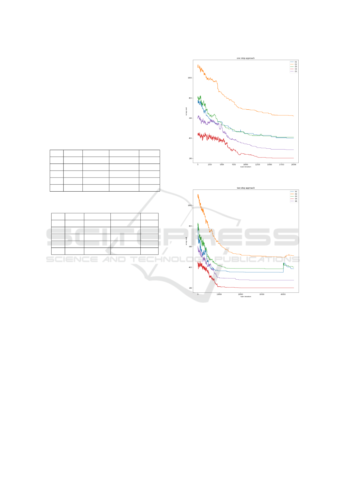
In the following ﬁgures we see the behaviour of the

scrap cost per iteration. In ﬁgure 1 the scrap cost de-

creases slowly as expected of SA1.

In ﬁgure 2 the scrap cost behaviour of SA2 is

shown. The sudden rise at the end indicates the sec-

ond step. Step one generates a good basis plan regard-

ing only scrap cost and the second step ﬁxes the con-

straint violations which on the other hand, partially

increased the scrap again.

6 CONCLUSION

In this article, a planning problem from the steel in-

dustry was presented, together with some typical rules

and constraints to be considered. We see that even to-

Figure 1: Shows the behaviour of the scrap cost over the

iterations from SA1.

Figure 2: Shows the behaviour of the scrap cost over the

iterations from SA2.

day, long-established optimization methods still pay

off. In this case the scheduling problem was mod-

elled as a well-studied TSP and a SA algorithm was

chosen to minimize the cost. Most of the time the

difﬁculty is to formulate the speciﬁc problems of the

factory and constraints into rules and constraints. If

this succeeds, we have shown that the constraints and

rules can be described by the object function and that

small changes to the SA algorithm can improve the

quality of the solutions and reduce the computation

time. It is also important to observe how such opti-

mization programs can eventually be integrated into

the running processes of a factory.

The work described in this article has been funded

by the European Union under Grant Agreement

Traveling Salesman Problem: A Case Study of a Scheduling Problem in a Steelmaking Plant

295

869886. The authors would like to thank Nico Herbig

for his important contributions in the initial problem

deﬁnition and modeling phase.

REFERENCES

Ascheuer, N. (1996). Hamiltonian path problems in the on-

line optimization of ﬂexible manufacturing systems.

PhD thesis.

Dahal, K., McDonald, J., and Burt, G. (2000). Modern

heuristic techniques for scheduling generator mainte-

nance in power systems. Transactions of the Institute

of Measurement and Control, 22(2):179–194.

Johnson, D. S. and McGeoch, L. A. (1997). The travel-

ing salesman problem: A case study in local opti-

mization. Local search in combinatorial optimization,

1(1):215–310.

Liu, S., Pinto, J. M., and Papageorgiou, L. G.

(2008). A tsp-based milp model for medium-

term planning of single-stage continuous multiproduct

plants. Industrial & Engineering Chemistry Research,

47(20):7733–7743.

Matai, R., Singh, S. P., and Mittal, M. L. (2010). Traveling

salesman problem: an overview of applications, for-

mulations, and solution approaches. Traveling sales-

man problem, theory and applications, 1.

Pasotti, A. and Zavanella, L. (2007). Implementing ad-

vanced scheduling techniques in industrial environ-

ments: evidences and outcomes.

Zhan, S.-h., Lin, J., Zhang, Z.-j., and Zhong, Y.-w. (2016).

List-based simulated annealing algorithm for traveling

salesman problem. Computational intelligence and

neuroscience, 2016.

ETCIIM 2022 - International Workshop on Emerging Trends and Case-Studies in Industry 4.0 and Intelligent Manufacturing

296