Enhancing the Geometry of Curvilinear Sections of the Track Plan

for High-speed Traffic

Sergey Shkurnikov

, Sergey Kosenko

and Olga Bulakaeva

Emperor Alexander I St. Petersburg State Transport University, St. Petersburg, Russian Federation

Siberian Transport University, Novosibirsk, Russian Federation

Keywords: Alignment plan, high-speed track, transition curves, curved section.

Abstract: The paper outlines the key trends in the current science of high-speed railways layout and profile design. The

employment of sophisticated laser scanning systems and satellite navigation systems simplifies the task of

constructing and maintaining complex spatial curves - areas of overlapping vertical curves in the profile and

transitional curves in the plan, sinusoidal or polynomial curves. As part of this research, a mathematical

model has been developed to describe different transition curves with non-linear curvature and elevation

characteristics of the outer rail depending on the number of zero derivatives required at the ends of the

transition curves. The shape influence (character of curvature function change within the transition curve) of

curvilinear sections of high-speed railway track plan on traffic dynamics is investigated. It has been found

that the best dynamic performance is in the curved section of the alignment equipped with transition curves

whose curvature function is represented by a 5th degree polynomial. There may also be no circular curve

within the plot in question. The paper examines the construction and mutual arrangement of differently shaped

curved sections and identifies their advantages and disadvantages.

1 INTRODUCTION

The requirements of the present development and

implementation phase of high-speed rail traffic in the

Russian Federation are shaping new approaches to the

design of the track plan and profile. As a result of

developments in the railway industry some provisions

previously considered fundamental and indisputable

are subject to critical rethinking.

The permissibility of overlapping transition and

vertical curves in the same alignment is limited by the

requirements of the existing regulatory framework

which has not lost its relevance for decades. When it

was formed in the 1960s this prohibition was justified

by the difficulty of maintaining a complex spatial

curve. However, the application of modern laser

scanning systems, GPS and GLONASS makes this

task easier. Compliance with the requirement for non-

conformity of vertical curves in the plan and

transition curves in the profile leads to an increase (up

to 33.8 % (Akkerman, 2017) in the construction cost

https://orcid.org/0000-0002-4273-389X

https://orcid.org/0000-0003-2987-1435

https://orcid.org/0000-0003-0982-5183

of high-speed railways (HSR). A maximum speed of

400 km/h can be realised by using large radius

vertical curves (30-40 km). The vertical curve length

is proportional to the radius, therefore longer

longitudinal profile elements are required to

accommodate vertical curves outside the transition

line which causes difficulties in routing and increases

the cost of highway construction (EN 13803-1:2010).

In order to improve the smooth running of trains

studies are being carried out on the possibility of

constructing a curve by interfacing two clothoids both

in plan and in track profile. The need for a straight

insertion between two adjacent curves in the plan,

assuming a "clothoidal" coupling, is also not obvious,

according to (Akkerman, 2017).

The regulatory value of unaccelerated speed

ensures passenger comfort when running a high-

speed train and indirectly determines the level of

permissible lateral impact of the rolling stock on the

track. In Russia the unaccelerated speed of 400 km/h

is 0,4 m/s

. This value is generally commensurate

200

Shkurnikov, S., Kosenko, S. and Bulakaeva, O.

Enhancing the Geometry of Curvilinear Sections of the Track Plan for High-speed Trafﬁc.

DOI: 10.5220/0011581700003527

In Proceedings of the 1st International Scientiﬁc and Practical Conference on Transport: Logistics, Construction, Maintenance, Management (TLC2M 2022), pages 200-206

ISBN: 978-989-758-606-4

 2023 by SCITEPRESS – Science and Technology Publications, Lda. Under CC license (CC BY-NC-ND 4.0)

with the requirements of European standards

(Lindahl, 2001; Sirong, 2018). Nevertheless, Russian

research on the basis of train tests has established an

unaccelerated speed limit of 1,0 m/s

for high-speed

and high-speed traffic due to the improved dynamic

qualities of high-speed rolling stock. An increase in

the regulatory value of unaccelerated acceleration up

to 0.75 m/s

has also been noted on PRC high-speed

roads (Sirong, 2018). Increasing the allowable rates

of unaccelerated speed leads to a reduction in the

required curve radius in the plan. On the one hand,

this ensures a better alignment with the terrain,

reduces the construction and maintenance costs of

very gentle curves and on the other hand it affects the

comfort of the journey and the quality of the service

provided.

A separate area of improvement in the geometry

of the HSR route is the definition of a rational shape

of the transition curves due to the nature of the spatial

variation in curvature within its length. In addition to

the transition curves with linearly varying curvature

(clothoids) traditional for the Russian Federation

international experience distinguishes sinusoidal

(Sine (EN 13803-1:2010), cosine (Cosine (EN

13803-1:2010) and polynomial (Wiener Bogen,

Bloss) transition curves (Hasslinger, 2005; Wojtczak,

2018; Velichko, 2020). The main disadvantage of

clothoidal transition curves is that there is significant

rolling stock oscillation when traversing curved

sections of the alignment at the junctions of straight

lines with transition curves and transition curves with

circular curves (Xiaoyan, 2017; Morozova, 2020).

The cause of oscillation, in terms of the laws of

mechanics, is the piecewise linear description of the

curvature function within the length of the section in

question. Negative dynamic impacts are considered to

be compensated for by rational assignment of

transition and circular curve lengths. However, the

increased demands on traffic dynamics on the HSR

lead to the need to select a rational transition curve

shape and to determine the conditions for their

applicability.

2 MAIN TEXT

2.1 Materials and Methods

The design of transition curves on railways has been

a major focus of domestic and foreign specialists

since the beginning of the twentieth century.

Proposals G. Schramm (1931) consisted in using

some composite curves as transition curves one of

which includes two centrally symmetric segments of

a 3rd-degree parabola (Helmert curve (EN 13803-

1:2010). In the case of curves of small radii, B.N.

Vedenisov suggested using only transition curves in

the form of transformed clothoids in the absence of

circular curves. Professor G.M. Shahunyants based

on the provisions of classical mechanics analysed the

change in progressive and rotational accelerations

arising from the movement of rolling stock in a curve.

Based on this analysis, G. M. Shahunyants developed

a transition curve whose 2nd derivative curvature

varies according to a sinusoidal law. A higher

requirement for smoothness of the curvature function

is suggested by V.P. Minorski. The curvature

function of the transition curve must comply with

four boundary conditions ensuring that the 1st, 2nd,

3rd and 4th derivatives of the curvature at the start

and end of the transition curve are zero.

As mathematical basis for the transition curves

considered in the present study we propose a

polynomial В

, defined on the interval [0; L

ТС

having at least one zero derivative on the ends of the

interval. It is assumed to grow monotonically and to

take В

min

= 0 и В

max

= 1 at its beginning and end

respectively calculated by the formula:

ВВ

=⋅







(1)

where В is a degree polynomial 1a − determined

from the condition:

1()

1(1) .

ТС

−

−+

∏

=+ −





















(2)

In equations (1) and (2) a is the multiplicity of the

node points which determines the degree of the

polynomial sought and is numerically equal to the

value k+1, k is the number of derivatives at the ends

of the segment set as zero; l is the current value of the

length of the transition curve and L

is the total

length of the transition curve (if k=0, then the

transition curve is represented as a clothoid).

The mathematical description of the function В

based on the theory of boundary conditions by V.P.

Minorsky assuming that the zero derivatives at the

ends of the segment can be more than 4. The

formation of the polynomial В

is realised by means

of an hermitian interpolation method.

The correlation between the function В

and the

curvature function k is provided by the condition:

Enhancing the Geometry of Curvilinear Sections of the Track Plan for High-speed Trafﬁc

201

(3)

The curvature and elevation of the outer rail must

coincide (proportionality):

(4)

In formulae (3) and (4) R is the radius of the

circular curve, H is the elevation of the outer rail in

the circular curve, k is the current curvature within

the transition curve, h is the current elevation of the

outer rail within the transition curve.

Transition curve lengths whose mathematical

description is based on the application of the В

function must comply with the conditions that the rate

of wheel lift [f] and the rate of increase of

unaccelerated acceleration [Ψ] do not exceed their

maximum values laid down in the regulations. It

should be noted that as the polynomial degree В

increases a lengthening of the transition curve is

required due to the magnitude of the curvature growth

rate (1st derivative of curvature) in the middle of the

transition curve. The dependence of the required

transition curve length L

ТС

on the polynomial degree

is shown in Figure 1.

In terms of the motion kinematics of a material

point on a curvilinear element the condition that the

first derivative of the curvature is zero (the third

derivative of the coordinate) at the start and end of the

transition curve is sufficient. This condition ensures

the continuity of the 'jerk' (the value ofψ on railways)

responsible for the reaction of passengers to changes

in acceleration and the safety of fragile goods. Large-

order derivatives are used quite rarely and do not even

have an approved name.

However, the movement of a railway carriage

within a curved section takes place simultaneously in

two planes: the horizontal transverse. The

translational motion and the vertical transverse - the

inclination of the carriage resulting from the ascent to

and descent from the elevation. The coordinates of the

vertical plane are proportional to the curvature. This

requirement allows the physical meaning to be

interpreted up to the third curvature derivative (the

fifth coordinate derivative):

− the first derivative of the curvature along the

length taking a zero value at the start and end

of the transition curve ensures continuity of the

additional force transient factors i, f и ψ, as well

as the angular velocity of the crew.

− the second deviation of the transition curve

turning to zero at the conjunctions with the

straight track and the circular curve ensuring

continuity of the angular acceleration.

− the third derivative of the curvature continuity

at the start and end of the transition curve

ensures that the angular acceleration rate

function or "jerk" in the vertical plane is

smooth.

2.2 Results and Discussion

2.2.1 Impact Studies of the Curved Track

Plan Shape on the Traffic Dynamics of

Highspeed Rolling Stock

The rolling stock dynamics during movement in

transition curves was investigated using a simulation

model of a high-speed vehicle (Wang, 2014) adapted

for the tasks of selecting design plan and route profile

parameters of high-speed railways using the

"Universal Mechanism" program.

A rolling stock simulation at 400 km/h was carried

out within a curved track element consisting of a

transition curve and a circular curve (R =

9400 m). The degrees of the polynomial В

, used to

describe the transition curves were varied from 1 to 5

within the framework of the numerical experiment

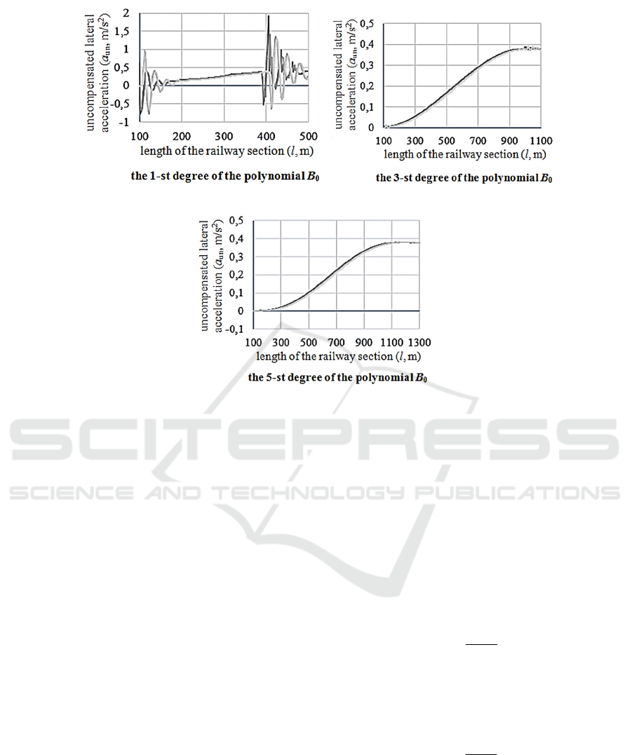
conducted. The experimental findings are shown in

Figure 2 in the form of oscillograms of unrecovered

transverse accelerations determined at the level of the

wheelset axle.

An examination of the results shows that the

maximum value of the unsuppressed transverse

acceleration (Zolotas, 2007) occurs at the interface

between the circular curve and the transition curve

Figure 1: Dependence of the required transition curve length on the degree of polynomial function В

TLC2M 2022 - INTERNATIONAL SCIENTIFIC AND PRACTICAL CONFERENCE TLC2M TRANSPORT: LOGISTICS,

CONSTRUCTION, MAINTENANCE, MANAGEMENT

202

a) b)

Figure 2: Oscillograms of lateral acceleration during high-speed rolling stock movement within differently shaped transition

curves.

whose curvature function is represented by a

polynomial of degree 1. The maximum actual value

of the unrelieved lateral acceleration

act.

unv.max

a is 2.0

m/s

and is several times greater than the calculated

value

сalc.

unv.max

(0.4 m/s

at a circular curve radius of

9400 m). Transition curves whose curvature function

is described by 3rd- and 5th-degree polynomials are

overcome without additional rolling stock

oscillations (

act.

unv.max

≈

сalc.

unv.max

The curved alignment shape is determined not

only by the degree of the transition curve polynomial

used to describe the curvature function but also by the

presence or absence of a circular curve. Figure 3

shows the simulation results for movement within

differently shaped curved sections.

According to the results obtained (Fig. 3 and Fig.

4) when organising high-speed rail traffic at 400 km/h

the best dynamic performance is in the curvilinear

section of the route plan equipped with transition

curves whose curvature function is represented by a

polynomial of degree 5. There may also be no circular

curve within the plot in question.

2.2.2 Features of the Arrangement and

Relative Positioning of Differently

Shaped Curvilinear Sections

A pie chart is developed to compare the device

requirements for non-linear curvature sections

arranged in series and traditional curvature:

− the minimum rotation angle

min

required to

construct a curved section of radius

R (sequence

of steps 1-2-3 in Figure 4);

min

(5)

−

Determination of the minimum radius

min

required to construct a curved section at a given

(sequence of steps 4-5-6 in Figure 4);

min

(6)

On the presented diagram Table 1 is filled in to

clearly evaluate the advantages and disadvantages of

the different shapes of the curved sections of the

alignment plan.

Enhancing the Geometry of Curvilinear Sections of the Track Plan for High-speed Trafﬁc

203

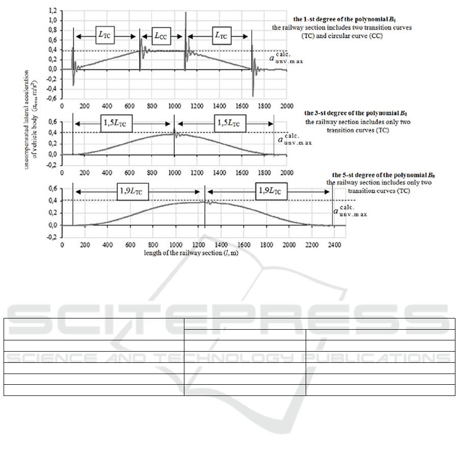
Figure 3: Magnitudes of unaccelerated acceleration in the crew bed occurring when driving within curved sections of different

shapes.

Table 1: Curved sections of different shapes.

Comparative characteristics

Swivel an

le 10°

nomial of de

ree 1

nomial of de

ree 5

Set / minimum radius of curved section, m 5000 5400

Length of transition curve, m 500 940

Total plot length, m 1373 1876

Length of constant curvature section, m 373

–

Bisector of the curved section, m 21 24

An obvious disadvantage of curvilinear sections

that include transition curves with a curvature

function described by a 5th degree polynomial is that

their length increases (1.36 times in the case in

question). However, for small alignment angles

(

α<α

min

) the required radius of the curved section

consisting of two transitional curves of non-linear

curvature increases thereby ensuring a reduction in

operating costs in the curve.

3 CONCLUSIONS

The result of this study allows us to change the usual

perceptions of the curved section of the high-speed

rail track plan. The best shape in terms of driving

dynamics is the curvilinear section within which the

additional oscillations of the crew tend to zero.

Equipping a curved section with transition curves

whose curvature and elevation divergence functions

are represented by5th degree polynomials meets these

requirements. The circular curve may not be present

at all in the section or may be smaller than the

standard value.

Despite better dynamic performance the length of

these transition curves is almost twice as long. It must

be taken into account that the permissible standard

values [

f] and [Ψ] have been determined for

clothoidal transition curves. It should be taking into

account the significant oscillations of the rolling stock

when passing through curved sections of the

alignment at the junctions of straight, transition and

circular curves. The implementation of transient

curves with non-linear curvature leads to the

complete damping of this kind of oscillation which

theoretically leads to an increase in the tolerance rates

[

f] и [Ψ]. Increasing these values contributes to

reducing the required length of the transition curves.

TLC2M 2022 - INTERNATIONAL SCIENTIFIC AND PRACTICAL CONFERENCE TLC2M TRANSPORT: LOGISTICS,

CONSTRUCTION, MAINTENANCE, MANAGEMENT

204

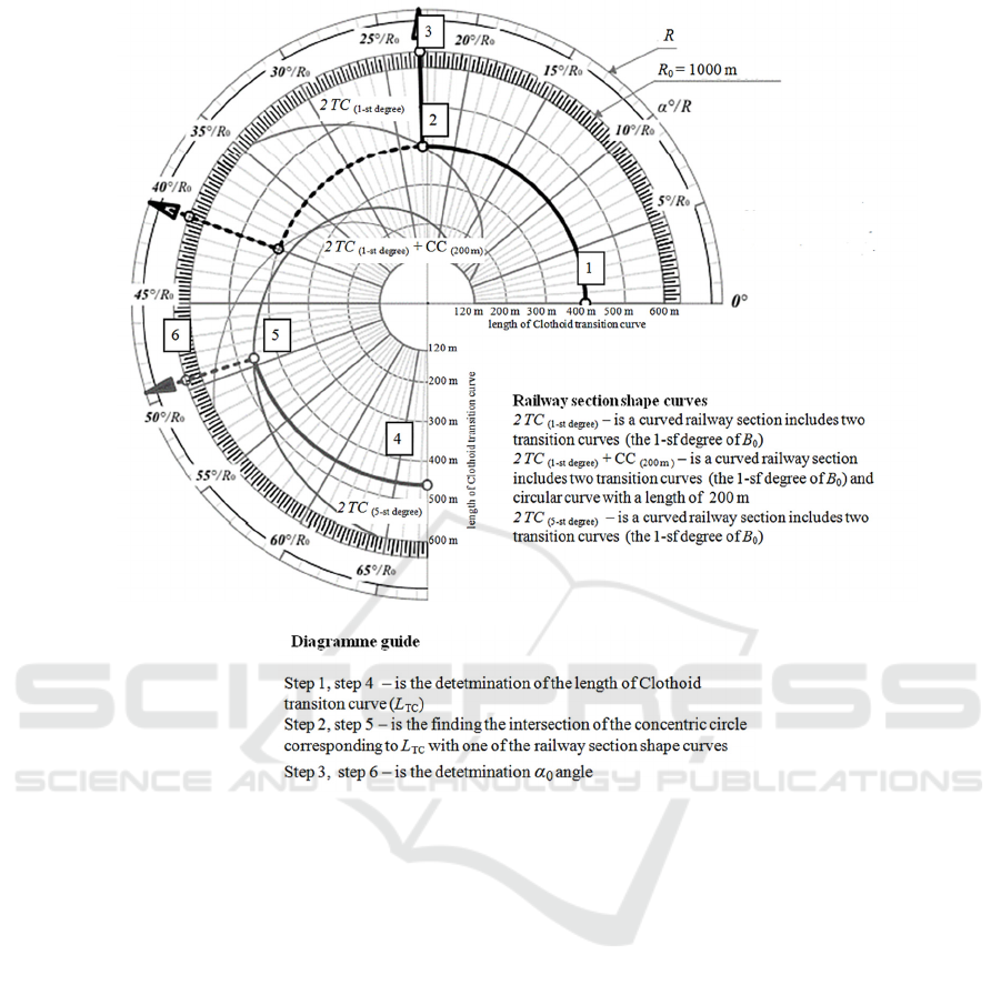
Figure 4: Pie chart for determining curvilinear section design features.

At the present stage of the study in the curvature

design of the high-speed railway alignment plan it is

recommended to replace the traditional curvature

sections with polynomial (

polynomial of degree 5)

transition curves, conjugate without circular curve in

cases of small alignment angles (

α<α

min

). For an

unbiased assessment of other design cases (

min

>α )

the installation of an experimental curvilinear section

and a train test to assess the possibility of increasing

the tolerances [

f] and [Ψ] is necessary.

REFERENCES

Akkerman, G. L., Akkerman, S. G., 2017. High-speed

railway highlights. Herald of the Ural State University

of Railway Transport. 2 (34). pp. 46-56.

EN 13803-1:2010: Railway applications – Track – Track

alignment design parameters – Track gauges 1435 mm

and wider - Part 1: Plain line [Required by Directive

2008/57/EC].

Lindahl, M., 2001. Track geometry for high-speed

railways: A literature survey and simulation of dynamic

vehicle response. Stockholm, TRITA-FKT Report,

Royal Institute of Technology. p. 160.

Sirong, Y., 2018. Dynamic analysis of high - speed railway

alignment: theory and practice. Academic Press. 324 p.

Hasslinger, H., 2005. Measurement proof for the

superiority of a new track alignment design element, the

so- called Viennese Curve” Berlin. ZEVrail. 129. pp.

61-71.

Wojtczak, R., 2018. General equation of cant ramp in form

of polynomial of odd degree.

https://www.researchgate.net/.

Wang, K., Zhai, W, 2014. Study on performance matching

of wheel-rail dynamic interaction on curved track of

speed-raised and high-speed railways. China Railway

Science, 35(1). pp. 142-144.

Velichko, G., 2020. Quality analysis and evaluation

technique of railway track + vehicle system

performance at railway transition sections with various

shape curves. Transport Means 2020 Proceedings of

the 24th International Scientific Conference Part II: pp.

573-578.

Enhancing the Geometry of Curvilinear Sections of the Track Plan for High-speed Trafﬁc

205

Xiaoyan, Lei, 2017. High speed railway track dynamics:

models, algorithms and applications. p. 414.

Long, X. Y., 2008. Study on dynamic effect of alignment

parameter on train running quality and its optimization

for high-speed railway.

Morozova, O. S., Shkurnikov, S. V., 2020. The

substantiation of design parameters of circular curves

on high-speed railways. Modern Technologies. System

Analysis. Modeling. 3 (67). pp. 152-159.

Zolotas, A. C., Goodall, R. M. Halikias, G. D., 2007. Recent

results in tilt control design and assessment of high

speed railway vehicles. Proc. ImechE Part F: J. Rail

and Rapid Transit. 221. pp. 291-312.

TLC2M 2022 - INTERNATIONAL SCIENTIFIC AND PRACTICAL CONFERENCE TLC2M TRANSPORT: LOGISTICS,

CONSTRUCTION, MAINTENANCE, MANAGEMENT

206