Heuristic Algorithm for 3D Modelling of a Railway Track Route
Nikita Dmitriev
a
Ural State University of Railway Transport, Yekaterinburg, Russia
Keywords: Heuristic algorithm, optimisation, railway track, plan modelling, profile modelling, terrain generation, digital
terrain model.
Abstract: A heuristic algorithm for 3-dimensional modelling of the railway route has been developed. In determining
the geometric parameters of the route, cost optimization was used, for which an asymmetric bell-shaped
function was introduced, having a minimum at the zero-work line and maximums in bridge and tunnel
construction. A gradual optimization technique is used as the main heuristic method, which consists of a
sequential solution of the optimization problem from the simplest cases to the most complex ones. The
increase in complexity occurs by dividing the segments of the alignment by a point whose coordinates undergo
a variation in three dimensions until the optimal cost is obtained. After iteration, the alignment is modified
according to current codes for railways, tunnels and bridges. The algorithm was tested on synthesized digital
elevation models using a modified diamond-square algorithm. The experimental investigation consisted in
variation of scaling factor of altitude matrix values. It was shown that the use of the developed algorithm leads
to finding a railway track route that differs in cost from the global optimum by not more than 5-15% on
average. The computational complexity of the constructed algorithm has a linear-logarithmic dependence on
the trajectory length.
1 INTRODUCTION
The design of the railway alignment takes place at the
strategic and tactical level. The strategic level
includes the tasks of implementing global economic
and social trends: it needs to understand which
settlements and logistics points should be involved in
order to optimise freight and passenger traffic flows.
Problems at the tactical level are those that arise after
a strategic decision has been taken: it is assumed that
the choice of transport network focal points has
already been made and is not negotiable. This level
includes the specific design of future railways,
bridges and tunnels, taking into account topography,
hydrology, geology and climate.
This study addresses the task of automatically
constructing a cost-optimal track in plan and profile
based on elevation information for a preliminary
economic justification of a future detailed design.
Focusing on relief is explained by the fact that even
with geometrically insignificant changes in the route
to be laid, there is a significant increase in
construction costs, resources used and road operation
due to the non-linearity of the cost function
a
https://orcid.org/0000-0002-6779-3442
(Ghoreishi, 2019). The possibility of adequate
functioning of algorithms in mountainous terrain is of
particular importance here, because the economic
result in stressed sections is several times greater than
the effect in free sections (Struchenkov, 2021).
To obtain information on relief and further
application of traditional cameral tracing, it is
possible to use digitized maps, e.g., topographic
maps. The basic elements of tracing are its projection
on a horizontal plane (plan) and a vertical section
along the projected line (longitudinal profile). When
tracing, the requirements of railway infrastructure
codes, railways, bridges and tunnels must be
complied with (Bushuev, 2019; Skutin, 2019). The
competing directions along which the alignment is
constructed are often chosen intuitively, based on the
past experience of the designers, which can lead to
different designers proposing different possible
solutions for the trajectory, which does not meet the
basic requirement of solving the optimisation
problem.
Manual tracing uses modern CAD, which often
allows the requirements on the nature of the trajectory
to be met, but does not take into account cost
136
Dmitriev, N.
Heuristic Algorithm for 3D Modelling of a Railway Track Route.
DOI: 10.5220/0011580300003527
In Proceedings of the 1st International Scientific and Practical Conference on Transport: Logistics, Construction, Maintenance, Management (TLC2M 2022), pages 136-142
ISBN: 978-989-758-606-4
Copyright
c
 2023 by SCITEPRESS – Science and Technology Publications, Lda. Under CC license (CC BY-NC-ND 4.0)

optimisation. Among domestic software products
performing some automation functions it is necessary
to mention Credo, RVPlan, Korwin, Robur, among
foreign ones – Civil 3D, GeoniCS, MXRAIL.
Nevertheless, the issue of building a software system
where it would be possible to select different
optimality criteria and the development would be
fully automated after the task of technical
specification and input of geoinformation data
remains almost unexplored. Currently, the operator is
left with such problems as calculating construction
and operating costs, maximum rail speed, fuel and
resources consumption, and train travel times along
the section. In some CAD, for example, Invest, the
economic calculations of the main elements of the
railway track are partially automated interactively. In
CAD Aquila (Bykov, 2017), the length of calculated
sections is limited to 15-25 km, which makes it
possible to perform economic justification only for
short sections of track.
The basic problem of the decision of a task of
automatic designing is not only a high degree of a
variability of a choice of geometrical sections
(straight lines, circular and transitive curves) and their
parameters, but also the quantity of these sections,
depending on mountainous terrain. All this leads to
the fact that the computational complexity of the
potential algorithm will be:
𝑇(𝑁) = 𝑂
(
2

)
=𝑂2




(1)
where N is the number of track elements, AB is point-
to-point distance between A and B, Rε – the minimum
size of a single trajectory section.
Nevertheless, such a variational approach is also
used in current research (Prokop’eva, 2017;
Kholodov, 2019; Sidorova, 2020), with a manual
method being implemented in automatic mode, often
separately in plan and separately in profile. However,
there are also emerging studies using new approaches
to trajectory generation, such as iterative approach
(Pu, 2021), fuzzy hierarchy analysis (Singh, 2019),
genetic (Kang, 2020; Li, 2017) and evolutionary
algorithms (Polyanskiy, 2021), and swarm
intelligence (Ghoreishi, 2019). The main idea of these
methods is to treat the railroad track as a set of critical
points, which allows implementing various
approximate algorithms, without being strongly
influenced by the variability of the geometric element
selection. At the same time, for example in (Sushma,
2020), it remains possible to design the whole road
network in parallel instead of a single trajectory.
2 MATERIALS AND METHODS
Real data for the algorithm under development can be
obtained from aerial photographs (Roshchin, 2021) or
directly from topographic maps (Dmitriev, 2019). In
this case, the data are digital elevation models
(DEM). The first method in itself is time consuming,
although it saves later on planning tracing, while the
second method can automatically obtain the relief
data, but only in existing maps. Therefore, this study
for completeness was carried out on generated DEMs
using the diamond-square fractal algorithm (Smelik,
2014), an example of which is shown in Fig. 1. It is
worth noting that the use of DEMs in the form of
polynomials of high powers from two variables even
with a long selection of coefficients does not give a
real representation of the earth's surface, although in
this case the problem of finding the optimal trajectory
is reduced to the solution of simple functional
equations.
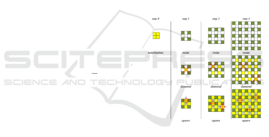
Figure 1: The first few steps of the diamond-square
algorithm.
The matrix 2×2 is initialised with zero values
before starting the algorithm. Then three actions are
performed for n times in sequence. First, the matrix
grid is scaled from the order of (2

+1) to the
order (2

+1) by adding null rows and columns
between the existing ones.
In step diamond for every four neighbouring
elements forming a square 3×3, the middle element is
initialised with the height value using the formula:
𝑧
(
𝑖,
𝑗
)
=0.25∗(𝑧
(
𝑖−1,
𝑗
−1
)
+𝑧
(
𝑖−1,
𝑗
+1
)
+
+𝑧
(
𝑖+1,
𝑗
−1
)
+𝑧
(
𝑖+1,
𝑗
+1
)
)+𝑅⋅𝑝

,
(2)
where (i, j) define the coordinates of the point under
study, z(i, j) is the height value, R∊[-1, 1] is a random
Heuristic Algorithm for 3D Modelling of a Railway Track Route
137

variable with a continuous uniform distribution,
p∊(0, 1) is a relief parameter, n is a step iteration
number.
The greater the parameter p, the more uneven the
terrain is. For the algorithm to work, a parameter
equal to the Golden Ratio was chosen, resulting in
good plausibility.
In step square a similar operation is performed,
but for every four neighbouring elements forming a
square rotated by 45 degrees. This may involve
referring to elements outside the existing matrix, in
which case zero is taken as the missing value. Then
the height value for the middle element is calculated
by the formula:
𝑧
(
𝑖,𝑗
)
=0.25∗(𝑧(𝑖−1,𝑗)+𝑧
(
𝑖,𝑗−1
)
+
+𝑧
(
𝑖,𝑗+1
)
+𝑧
(
𝑖+1,𝑗
)
)
+𝑅⋅𝑝

.
(3)
In general, the elevation values in the matrix can
take values of different meanings that are unrelated to
the real values, so the final matrix after n steps can be
transformed by performing linear operations, median
filtering and normalization. Elevations and troughs
with random characteristics were added to the final
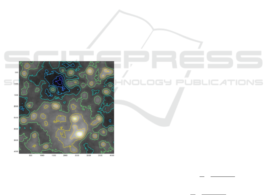
elevation map to increase plausibility. An example of
the resulting digital map together with the contour
lines is shown in Figure 2.
Figure 2: Example of a digital map obtained; brightness
corresponds to height.
The total construction cost can be calculated using
the formula for the economic justification of the
proposed track trajectory:
𝐶𝑜𝑠𝑡(𝐿)
=𝑐(𝑥(𝑡),𝑦(𝑡), 𝑧(𝑡) −𝑧

(𝑥(𝑡),𝑦(𝑡)))𝑑𝑙

,
(4)
where L is a curve in three-dimensional space, x(t),
y(t), z(t) define its parametric representation using
Cartesian coordinates, t∊[0, 1] is a parameter for
which zero corresponds to the start of the trajectory,
one to the end, с(x, y, Δz) is a unit cost function, z
DEM
is an elevation values from a digital elevation model.
Although in the general case it is the integral that
must be calculated, since the map is a discrete square
matrix, it is possible to go from calculating the
integral to the sum:
𝐶𝑜𝑠𝑡(𝐿)= 𝑐(𝑥

,𝑦

,𝑧

−𝑧

(𝑥

,𝑦

)) ⋅ 𝐿

.


(5)
We construct a mathematical model of the unit
cost function based on the following conditions:
a) at ∆z = 0 it takes the value с0, which
corresponds to the line of zero work;
b) at ∆
+
crit
> ∆z >0, it is quadratic around zero,
which corresponds to an increase in the cross-
sectional area of the required embankments;
c) at ∆z > ∆
+
crit
, it takes the value M
+∞
>> c0,
which corresponds to the construction of a bridge
with a cost that does not depend on its height;
d) at ∆
-
crit
< ∆z < 0, it has a quadratic character
around zero (but with a different coefficient), which
corresponds to an increase in the cross-sectional area
of the required excavation;
e) at ∆z < ∆
-
crit
, it takes the value M-
∞
>> c0, which
corresponds to the construction of a tunnel that is not
dependent on the depth of the tunnel;
f) the function should have a smooth transition
between b-c and d-e to avoid complicating the design
with separate bridge and tunnel sections at this stage.
All presented parameters can vary considerably
for different soils, the study assumes that they are
equal for the given site. Point c may also not be
fulfilled at certain bridge designs. The study assumes
that all railway alignments are of the same type.
Considering these points and the conditions for
the specific cost function at a point, a mathematical
model of the asymmetric bell-shaped function has
been derived:
𝑐
(
𝑥,𝑦,𝛥𝑧
)
=𝜃
(
𝛥𝑧
)
∗
с

2
+
𝑀

⋅𝛥

𝑧
𝜎


+𝛥

𝑧
+
+𝜃(−𝛥𝑧) ∗ 
с

2
+
𝑀

⋅𝛥

𝑧
𝜎


+𝛥

𝑧
,
(6)
where θ(x) is the Heaviside function, с0 defines track
cost along the zero-work line, M
+∞
, M-
∞
are the costs
for bridge and tunnel construction respectively, σ
+∞
,
σ
-∞
are the parameters defining the critical value Δz,
where the strategy is changed to building a bridge or
tunnel. Although the Heaviside function θ(x) has a
TLC2M 2022 - INTERNATIONAL SCIENTIFIC AND PRACTICAL CONFERENCE TLC2M TRANSPORT: LOGISTICS,
CONSTRUCTION, MAINTENANCE, MANAGEMENT
138

discontinuity at a point x = 0, the specific cost
function c will be smooth, since its derivative has no
discontinuity at a given point.
Thus, to solve the trajectory optimization problem
between two points A and B, it is necessary to find
the functions x(t), y(t), z(t) satisfying the following
conditions:
𝐶𝑜𝑠𝑡(𝐿

)→𝑚𝑖𝑛,
𝑥(0) = 𝑥

,𝑦(0)=𝑦

,𝑧(0)=𝑧

,
𝑥(1) = 𝑥

,𝑦(1)=𝑦

,𝑧(1)=𝑧

.
(7)
In addition, the restrictions expressed in the codes
of practice should be complied with, e.g., for the
railways of 1520 mm gauge (PC 119.13330.2017),
tunnels (PC 122.13330.2012) and bridges (PC
46.13330.2012). The main features which are most
affected by topography and which must be taken into
account when tracing a railway are the maximum
track gradient, the minimum curvature radius in the
plan and the minimum gradient in tunnels.
Any discrete elevation matrix can be converted to
analytical form by interpolation, e.g., by Lagrange
polynomials. At that, the functions with the number
of parameters equal to the number of DEM elements
will be analysed, which will lead to high
computational complexity. For example, the DEM
used below has the number of elements of the order
of 65 million. It is worth noting that this method does
not ensure that the railway requirements are met. If
local interpolation is used, for example bicubic
interpolation, it will not be possible to apply
variational calculus methods to the entire map set.
Another approach is to represent the three-
dimensional space as a uniform graph with N levels
of discretization along each of the axes. Thus, the
number of vertices in this graph will be N
3
, and the
number of edges depends on the connectivity. For
example, a Von Neumann neighbourhood connects
only cells that have a common side, while a Moore
neighbourhood also connects common vertices.
Applying graph theory and graph traversal methods,
such as Dijkstra's algorithm, it is possible to obtain a
path of minimum length. The computational
complexity of such an algorithm will be O(N
6
), which
is already large enough for a number of sampling
levels on the order of 1000, corresponding to a small
DEM of 1MB size. The algorithm A* generally uses
an exponential number of points relative to the path
length, which is also not practical in this case.
Nevertheless, it is not necessary to obtain a strictly
optimal solution if large computational power is
needed. For example, if a trajectory that differs by
only a few percent from the optimal cost in a
sufficient amount of time is obtained, this would also
be an acceptable result.
One class of algorithms that have the property of
quickly finding a solution, albeit not the most optimal
one, but a good one, is heuristics. One of the heuristic
methods is the technique of gradual optimization.
Then a difficult optimization problem is solved first
for a much-simplified problem, gradually increasing
the complexity until the complexity equals the initial
one. The intermediate results should be less and less
different with each step: when this change stops or
becomes less than some threshold, the heuristic
algorithm stops.
At step zero, the trajectory is an AB segment. To
implement the iterative steps of the algorithm, we
should note the existence of invariants for passing any
trajectory from A to B, including the optimal
trajectory. If we need to connect two points in three-
dimensional space with a curve, then it should in any
case intersect some set of planes. One of such planes
is the plane perpendicular to the given segment and
passing through its middle. Assuming that points A
and B are not above each other, which is adequate for
the problem, then such a plane is also the plane
perpendicular to the horizontal plane and to the
segment AB in the plane plan. Correspondingly, we
will select a new point exactly in this plane, using the
parametric definition of the planes:
𝑥

=
𝑥

+𝑥

2
+
𝑦

−𝑦

2
⋅𝑅

,
𝑦

=
𝑦

+𝑦

2
−
𝑥

−𝑥

2
⋅𝑅

,
𝑧

=
𝑧

+𝑧

2
+
𝑧

−𝑧

2
⋅𝑅

,
(8)
where R
1
and R
2
are random variables having a
continuous uniform distribution and specifying the
variation, z
high
and z
low
are the boundary heights,
which can be iteratively calculated as follows:
𝑧

=𝑚𝑖𝑛(𝑧

+𝑖
р
⋅𝐴𝐶,𝑧

+𝑖
р
⋅𝐵𝐶,𝑚𝑎𝑥(𝑧

,𝑧

)),
𝑧

=𝑚𝑎𝑥(𝑧

−𝑖
р
⋅𝐴𝐶,𝑧

−𝑖
р
⋅𝐵𝐶,𝑚𝑖𝑛(𝑧

,𝑧

)),
(9)
where i
р
– the value of the maximum gradient. First,
the heights at points A and B are selected as
boundaries, then the boundary values are recalculated
with the new value z
C
. At larger distances, the
boundary values resulting from the maximum
gradient are chosen more often, and at small
distances, the elevation values at points A and B
remain.
To select the correct variation, it is necessary to
calculate the value of the alignment along the ACB
polygon, which can be done in O(L
ACB
) operations. It
Heuristic Algorithm for 3D Modelling of a Railway Track Route
139

can be assumed that the cost calculation for each
broken line is approximately the same and its time
complexity belongs to the class O(L). In the next
iterations the heuristic algorithm is repeated, but
already for new pairs of points AC and CB,
generating new two points, then 4 segments are
investigated, in the next step 8 and so on.
We assume a difference in the number of
variations of points at each separate step: let the j-th
iteration of the algorithm be v
j
variations, then the
complexity of the algorithm after the nth iteration will
belong to the class 𝑂
∑
𝑣

⋅2

⋅𝐿


. Thanks to
the formulas, any point on the map can be chosen as
the midpoint. This naturally reduces both the size of
the segments in question (at least as much as
√
2
), as
well as the area over which variation can occur (by at
least a factor of 2). In order to maintain the density of
variations per unit area, the number of variations can
be taken as 𝑣

=𝑣/2

, which will simplify the
computational complexity to a class of 𝑂
(
𝑣⋅𝑛⋅𝐿
)
.
Taking into account the discrete nature of the
resulting trajectory, it can be noted that the length of
the optimal trajectory is equal to the number of points
on it. The number of iterations before reaching
segments of length one is asymptotically equal to
𝑂(𝑙𝑔𝐿). As a result, the complexity class of the
algorithm presented is 𝑂
(
𝐿⋅𝑙𝑔𝐿
)
, which allows to
use elevation maps of practically any size and
accuracy, as the constructed algorithm will work in
linear-logarithmic time from DEM diameter.
The developed algorithm naturally uses the nature
of three-dimensional space, implementing
modification of points in parallel along all axes,
which can also be used to speed up calculations on
several processor cores. In addition, the possibility of
increasing the number of points to the order of O(L)
is assumed, that on the one hand increases the used
memory, but allows with more confidence to find the
global optimum, than a limited number of points, as
in the algorithms of collective intelligence. All points
obtained in each subsequent step are based on the
problem already solved for a smaller number of
points.
To analyse the bridge and tunnel constraints, we
study the resulting profile. If there will be two
elements of the same type next to each other, e.g., two
tunnels with a small crossing, they should be merged
into one. At correcting the elevation values at the
element boundaries, the slope in these areas may
exceed the allowable slope, so it is necessary to
normalize it, which will lead to a system error. In this
case the global optimum may be lost, but the number
of such special sections is not that large relative to the
total length of the alignment, which is accounted for
by bridges and tunnels.
Next, it is necessary to correct the sections with
small curvature radii by replacing them with curves
of larger radius. To do this, a straightening operation
is performed for each of the three critical points:
𝑥

:=
1
2
𝑥

+
𝑥

+𝑥

2
,
𝑦

:=
1
2
𝑦

+
𝑦

+𝑦

2
.
(10)
Since the plan and profile points have been
corrected, the optimization algorithm should be run
again, but without adding new points. In any case
these corrections do not take more than O(L) time, so
they do not affect the total computational complexity.
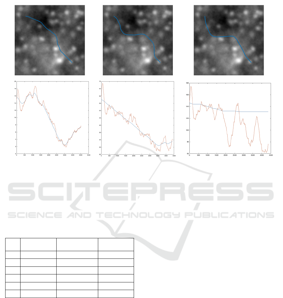
3 RESULTS
The pseudo planetary relief generation and the
heuristic automatic tracing algorithm have been
implemented as software in the MatLab package. The
quality of the generated data can be adjusted by
specifying the number of steps of the diamond-square
algorithm and its parameters. Each DEM element was
matched to a 1 m
2
square. Modifications to the
algorithm increased the confidence of the generated
terrain.
As a computational experiment, the task of
modelling a railroad track in plan and profile from
point A to B was set for the elevation map presented
above, the values in which are scaled with factor m
for the relief degree task from near plain, to
mountains. This experimental study raises the
question, for which type of terrain would it be most
difficult to construct an optimal trajectory? The
following parameters were chosen: i
р
= 10‰, i
min
=
3‰, R
min
= 500 m. The cost model parameters are: c0
= 1, M
+∞
= 10, σ
+∞
= 10 m, M
-∞
= 20, σ
-∞
= 20 m. The
results for the different coefficients m are shown in
Figure 3.
The lowest possible cost arises when there is no
relief between points A and B of the smaller steering
slope, when the optimum trajectory and is a segment
AB running along the line of zero work. This value is
unattainable because some relief always exists. In
addition, the study also aims at solving the problem
of designing a railway track in difficult terrain
conditions. Nevertheless, this value is very
convenient because it is possible to count the
effectiveness of the constructed path optimisation in
units of Cost
min
. To investigate the stability of the
TLC2M 2022 - INTERNATIONAL SCIENTIFIC AND PRACTICAL CONFERENCE TLC2M TRANSPORT: LOGISTICS,
CONSTRUCTION, MAINTENANCE, MANAGEMENT
140

algorithm and the quality of its performance, the
algorithm was run 50 times on average for each value
of the scaling factor. The calculated stability indices
are shown in the Table 1.
Table 1: Stability indices of the developed heuristic
algorithm depending on the scaling factor m.
m
Average
value Cost
Standard
deviation Cost
Optimal
value Cost
30 1.17 0.07 1.11
60 1.32 0.09 1.26
90 1.59 0.11 1.51
120 1.80 0.32 1.53
150 3.03 0.65 2.57
300 13.05 1.57 12.06
4 DISCUSSION AND
CONCLUSION
It can be concluded that the developed and
implemented heuristic algorithm can be used to carry
out an initial economic justification of the chosen
direction, trajectory and route elements. The
exception is considered to be the areas with very high
mountainous terrain, or if it is necessary to solve the
problem for two points that are quite close in plan but
have quite a big difference in elevation, which leads
to insufficient use of the existing DEM to implement
a more complex bypass trajectory. Reducing the cost
of constructing the railway alignment will not only
lead to a reduction in labour costs, but also in the
resources used, including during operation. Further
research can focus on optimizing the algorithm to
reduce computational complexity, adding constraints
on the geometric parameters of the alignment, and
using parallel computing. It is possible to create a
more stable algorithm, the results of which will not be
so strongly affected by the variations arising from the
use of random variables.
Analysis of statistical data shows an increase in
the average value of the cost with an increase in
mountainous terrain, at that the optimum value grows
more slowly than the algorithm average. First of all,
this means that there is a much greater amount of
variation with increasing terrain topography, causing
the algorithm to drift further away from finding the
global optimum. At further growth of the scaling
factor, the average value of the cost again approaches
the optimum, as it becomes easier to make the choice
at sufficiently high elevations, which illustrates the
effect when rigid nonlinearities are given by
mathematical formulas that are simpler to analyse.
Figure 3: Model of the railway line in plan (above) and longitudinal profile (below) as a function of depending on the scaling
factor, from left to right: m = 30; m = 120; m = 300.
Heuristic Algorithm for 3D Modelling of a Railway Track Route
141

REFERENCES
Ghoreishi, B., Shafahi, Y., Hashemian, S. E., 2019. A
model for optimizing railway alignment considering
bridge costs, tunnel costs, and transition curves. Urban
Rail Transit. 5(4). pp. 207–224.
Struchenkov, V. I., Karpov, D. A., 2021. Two-stage spline-
approximation with an unknown number of elements in
applied optimization problem of a special kind.
Mathematics and Statistics. 9(4). pp. 411–420.
Bushuev, N. S., 2019. Design aspects of railway lines in
permafrost conditions. Modern Technologies. System
Analysis. Modeling. 63(3). pp. 135–142.
Skutin, A. I., Kasimov, M. A., 2019. Peculiar features of
designing railway high-speed mainlines for passenger
traffic in conditions of the Ural region. Innotrans.
3(33). pp. 46–49.
Bykov, Y. A., Buchkin V. A., 2017. Prospects for the
development of railway transport corridors between
Europe and Asia and the methodology for their
multicriteria evaluation. Quality Management,
Transport and Information Security, Information
Technologies. 80857632017. pp. 66–68.
Prokop'eva, O. A., Zhuravskaya, M. A., 2017. On the issue
of creating energy-saving elements of the transport and
logistics infrastructure on the example of biclottoid
projecting. Innotrans. 1(23), pp. 3–7.
Kholodov, P. N., Titov, K. M., Podverbnyi, V. A., 2019.
Modelling the railway track plan and its changes during
the operation process. Modern technologies. System
analysis. Modelling. 1(61). pp. 74–85.
Sidorova, E. A., Vaganova, O. N., Slastenin, A. Yu., 2020.
Methods for determining the position of the curve in the
plan and the influence of the geometry of the track on
the indicators of interaction between the track and the
rolling stock. Rus. Railway Scie. 79(6). pp. 365–372.
Pu, H., 2021. Optimization of grade-separated road and
railway crossings based on a distance transform
algorithm. Eng. Optimization. 54(2). pp. 232–251.
Singh, M. P. P., Singh, P., 2019. Fuzzy AHP-based multi-
criteria decision-making analysis for route alignment
planning using geographic information system (GIS).
Journal of Geographical Systems. 21(3). pp. 395–432.
Kang, M.-W., Schonfeld, P., 2020. Artificial intelligence in
highway location and alignment optimization:
Applications of genetic algorithms in searching,
evaluating, and optimizing highway location and
alignments, World Scientific. p. 288.
Li, W., 2017. Mountain railway alignment optimization
with bidirectional distance transform and genetic
algorithm. Computer-Aided Civ. and Infr. Eng. 32. pp.
691–709.
Polyanskiy, A. V., 2021. Railroad track technological
construction process modelling and optimization using
a genetic algorithm. Rus. J. of Transport Eng. 1(8). pp.
37.
Sushma, M. B., Maji, A., 2020. A modified motion
planning algorithm for horizontal highway alignment
development. Computer-Aided Civ. and Infrast. Eng.
35(8). pp. 818–831.
Roshchin, D. A., 2021. Improving the accuracy of forming
a digital terrain model along a railway track.
Measurement Techniques. 64(2). pp. 100–108.
Dmitriev, N., 2019. Complex method of reconstruction of
contour lines. AIP Conference Proceedings 45th
International Conference on Application of
Mathematics in Engineering and Economics. 217213.
Smelik, R. M., 2014. A survey on procedural modelling for
virtual worlds. Computer Graphics Forum. 33(6). pp.
31–50.
TLC2M 2022 - INTERNATIONAL SCIENTIFIC AND PRACTICAL CONFERENCE TLC2M TRANSPORT: LOGISTICS,
CONSTRUCTION, MAINTENANCE, MANAGEMENT
142