Training Neural Networks in Single vs. Double Precision

Tomas Hrycej, Bernhard Bermeitinger

and Siegfried Handschuh

Institute of Computer Science, University of St. Gallen (HSG), St. Gallen, Switzerland

Keywords:

Optimization, Conjugate Gradient, RMSprop, Machine Precision.

Abstract:

The commitment to single-precision ﬂoating-point arithmetic is widespread in the deep learning community.

To evaluate whether this commitment is justiﬁed, the inﬂuence of computing precision (single and double

precision) on the optimization performance of the Conjugate Gradient (CG) method (a second-order optimiza-

tion algorithm) and Root Mean Square Propagation (RMSprop) (a ﬁrst-order algorithm) has been investigated.

Tests of neural networks with one to ﬁve fully connected hidden layers and moderate or strong nonlinearity

with up to 4 million network parameters have been optimized for Mean Square Error (MSE). The training

tasks have been set up so that their MSE minimum was known to be zero. Computing experiments have dis-

closed that single-precision can keep up (with superlinear convergence) with double-precision as long as line

search ﬁnds an improvement. First-order methods such as RMSprop do not beneﬁt from double precision.

However, for moderately nonlinear tasks, CG is clearly superior. For strongly nonlinear tasks, both algorithm

classes ﬁnd only solutions fairly poor in terms of mean square error as related to the output variance. CG

with double ﬂoating-point precision is superior whenever the solutions have the potential to be useful for the

application goal.

1 INTRODUCTION

In the deep learning community, the use of sin-

gle precision computing arithmetic (the ﬂoat32 for-

mat) became widespread. This seems to result from

the observation that popular ﬁrst-order optimization

methods for deep network training (steepest gradi-

ent descent methods) do not sufﬁciently beneﬁt from

a precision gain if the double-precision format is

used. This has even led to a frequent commitment

to hardware without the capability of directly per-

forming double-precision computations. For convex

minimization problems, the second-order optimiza-

tion methods are superior to the ﬁrst-order ones in

convergence speed. As long as convexity is given,

their convergence is superlinear –– the deviation from

the optimum in decimal digits decreases as fast as or

faster than the number of iterations. This is why it is

important to assess whether and how far the accuracy

of the second-order methods can be improved by us-

ing double precision computations (that are standard

in many scientiﬁc and engineering solutions).

https://orcid.org/0000-0002-2524-1850

https://orcid.org/0000-0002-6195-9034

2 SECOND-ORDER

OPTIMIZATION METHODS:

FACTORS DEPENDING ON

MACHINE PRECISION

Second-order optimization methods are a standard

for numerical minimization of functions with a sin-

gle local minimum. A typical second-order method

is the Conjugate Gradient (CG) algorithm (Fletcher

and Reeves, 1964). (There are also attempts to de-

velop dedicated second-order methods, e.g., Hessian-

free optimization (Martens, 2010).) In contrast to the

ﬁrst-order methods, it modiﬁes the actual gradient in

a way such that the progress made by previous de-

scent steps is not spoiled in the actual step. The algo-

rithm is stopped if the gradient norm is smaller than

some predeﬁned small constant. CG has the prop-

erty if previous descent steps have been optimal in

their descent direction, that is if a precise minimum

has been reached in this direction. This is reached by

a one-dimensional optimization subroutine along the

descent direction, called line search. Line search suc-

cessively maintains three points along this line, the

middle of which has a lower objective function value

than the marginal ones. The minimization is done by

shrinking the interval embraced by the three points.

Hrycej, T., Bermeitinger, B. and Handschuh, S.

Training Neural Networks in Single vs. Double Precision.

DOI: 10.5220/0011577900003335

In Proceedings of the 14th International Joint Conference on Knowledge Discovery, Knowledge Engineering and Knowledge Management (IC3K 2022) - Volume 1: KDIR, pages 307-314

ISBN: 978-989-758-614-9; ISSN: 2184-3228

307

The stopping rule of line search consists in specifying

the width of this interval at which the minimum has

been reached with sufﬁcient precision. The precision

at which this can be done is limited by the machine

precision. Second-order methods may suffer from in-

sufﬁcient machine precision in several ways related to

the imprecision of both gradient and objective func-

tion value computation:

• The lack of accuracy of the gradient computation

may lead to distorted descent direction.

• It may also lead to a premature stop of the algo-

rithm since the vanishing norm can be determined

only with limited precision.

• It may lead to wrong embracing intervals of line

search (e.g., with regard to the inequalities be-

tween the three points).

• It may also lead to a premature stop of line search

if the interval width reduction no longer succeeds.

There are two basic parameters to control the com-

putation of the CG optimization: There is a thresh-

old for testing the gradient vector for being close to

zero. This parameter is usually set at a value close to

the machine precision, for example, 10

−7

for single-

precision and 10

−14

for double-precision. The only

reason to set this parameter to a higher value is to tol-

erate a less accurate solution for economic reasons.

Another threshold deﬁnes the width of the interval

embracing the minimum of line search. Following the

convexity arguments presented in (Press et al., 1992),

this threshold should not be set to a lower value than

a square root of machine precision to prevent use-

less line search iterations hardly improving the min-

imum. Its value is above 10

−4

for single precision

and 3 ×10

−8

for double precision (Press et al., 1992).

There may be good reasons to use even higher thresh-

olds: low values lead to more line search iterations per

one gradient iteration. Under overall constraints of

computing resources such as limiting the number of

function calls, it may be more efﬁcient to accept a less

accurate line search minimum, gaining additional gra-

dient iterations. The experiments have shown that the

inﬂuence of the tolerance parameter is surprisingly

low. There is a weak preference for large tolerances.

This is why the tolerance of 10

−1

has been used for

both single and double precision in the following ex-

periments. The actual inﬂuence in the typical neural

network optimization settings can be evaluated only

experimentally. To make the results interpretable, it

is advantageous to use training sets with known min-

imums. They can be generated in the following way:

1. Deﬁne a neural network with speciﬁed (e.g., ran-

dom) weights.

2. Deﬁne a set of input values.

3. Determine the output values resulting from the

forward pass of the deﬁned network.

4. Set up a training set consisting of the deﬁned input

values and the corresponding computed results.

This training set is guaranteed to have a minimum er-

ror of zero.

3 CONTROLLING THE EXTENT

OF NONLINEARITY

It can be expected that the inﬂuence of machine pre-

cision depends on the problem. The most important

aspect is the problem size. Beyond this, the inﬂuence

can be different for relatively easy problems close to

convexity (nearly linear mappings) on one hand and

strongly non-convex problems (nonlinear mappings).

This is why it is important to be able to generate prob-

lems with different degrees of non-convexity. The

tested problems are feedforward networks with one,

two, or ﬁve consecutive hidden layers, and a linear

output layer. The bias is ignored in all layers. All

layers are fully connected. For the hidden layers, the

symmetric sigmoid with unity derivative at x = 0 has

been used initially as the activation function:

1 + e

−2x

−1 (1)

Both input pattern values and network weights

used for the generation of output patterns are drawn

from the uniform distribution. The distribution of in-

put values is uniform on the interval

a, b

−1, 1

whose mean value is zero and variance is

−a

3(b −a)

(2)

To control the degree of nonlinearity during train-

ing data generation, the network weights are scaled

by a factor c so that they are drawn from the uniform

distribution

−c, c

. The variance of the product of an

input variable x and its weight w is

−c

−1

(wx)

dxdw =

−c

(3)

For large N, the sum of N products w

converges

to the normal distribution with variance N

and stan-

dard deviation

√

. This sum is the argument of the

KDIR 2022 - 14th International Conference on Knowledge Discovery and Information Retrieval

308

sigmoid activation function of the hidden layer. The

degree of nonlinearity of the task can be controlled

by a normalized factor d such that c =

√

, resulting

in the standard deviation

of the sigmoid argument.

In particular, it can be evaluated which share of acti-

vation arguments is larger than a certain value. Con-

cretely, about twice the standard deviation or more is

expected to occur in 5 % of the cases.

If a sigmoid function in form eq. (1) is directly

used, its derivative is close to zero with values of in-

put argument x approaching 2. For normalizing factor

d = 2, the derivative is lower than 0.24 at 5 % of the

cases, compared to the derivative of unity for x = 0.

For normalizing factor d = 4, the derivative is lower

than 0.02 at 5 % of the cases. The vanishing gradient

problem is a well-known obstacle to the convergence

of the minimization procedure. The problem can be

alleviated if the sigmoid is supplemented by a small

linear term deﬁning the guaranteed minimal deriva-

tive.

(1 −h)



1 + e

−2x

−1



+ hx (4)

For such sigmoid without saturation with h =

0.05, the derivatives are more advantageous: For nor-

malizing factor d = 2, the derivative is lower than 0.28

at 5 % of the cases, compared to the derivative of unity

for x = 0. For normalizing factor d = 4, the derivative

is lower than 0.07 at 5 % of the cases.

This activation function eq. (4) is used for the

strongly nonlinear training scenarios.

4 COMPARISON WITH

RMSPROP

In addition to comparing the performance of the CG

algorithm (as a representative of second-order opti-

mization algorithms) with alternative computing pre-

cisions, it is interesting to know how competitive

the CG algorithm is compared with other popular

algorithms (mostly ﬁrst-order). Computing experi-

ments with the packages TensorFlow/Keras (Tensor-

Flow Developers, 2022; Chollet et al., 2015) and var-

ious default optimization algorithms suggest a clear

superiority of one of them: Root Mean Square Prop-

agation (RMSprop) (Hinton, 2012). In fact, this al-

gorithm was the only one with performance compara-

ble to CG. Other popular algorithms such as Stochas-

tic Gradient Descent (SGD) were inferior by several

orders of magnitude. This makes a comparison rel-

atively easy: CG is to be contrasted to RMSprop.

RMSprop modiﬁes the simple ﬁxed-step-length gra-

dient descent by adding a scaling factor

t,i

depend-

ing on the iteration t and the network parameter ele-

ment index i.

t+1,i

= w

t,i

−

t,i

∂E (w

t,i

)

∂w

t,i

= gd

t−1,i

+ (1 −g)



∂

E (w

t−1,i

)

∂w

t−1,i



(5)

This factor corresponds to the weighted norm of the

derivative sequence of the given parameter vector el-

ement. In this way, it makes the steps of parame-

ters with small derivatives larger than those with large

derivatives. If the convex error function is imagined

to be a “bowl”, it makes a lengthy oval bowl more cir-

cular and thus closer to a normalized problem. It is

a step toward the normalization done by CG but only

along the axes of individual parameters, not their lin-

ear combinations.

5 COMPUTING RESULTS

The CG method (Press et al., 1992) with Brent line

search has been implemented in C and applied to the

following computing experiments. It has been veri-

ﬁed by form published in (Nocedal and Wright, 2006)

(implemented in the scientiﬁc computing framework

SciPy (Virtanen et al., 2020)), with the line search al-

gorithm from (Wolfe, 1969).

Amendments of CG dedicated to optimize neural

networks have also been proposed: K-FAC (Martens

and Grosse, 2015), EKFAC (George et al., 2021),

or K-BFGS (Ren et al., 2022). They may possibly

improve the performance of CG in comparison to

RMSprop.

All training runs are optimized with a limit of

3,000 epochs for tasks with up to four million pa-

rameters. Smaller tasks had around 30,000, 300,000,

and 1 million parameters. The conﬁguration of the

reported largest networks with one or ﬁve hidden lay-

ers can be seen in table 1. The mentioned epoch limit

cannot be satisﬁed exactly since the CG algorithm al-

ways stops after a complete conjugate gradient itera-

tion and thus a complete line search could consist of

multiple function/gradient calls. The number of gra-

dient calls is generally variable per one optimization

iteration, however, during the experiments they were

always evaluated as often as forward passes.

The concept of an epoch in both types of experi-

ments corresponds to one optimization step through

the full training data with exactly one forward and

one backward pass. For CG, the number of for-

ward/backward passes can vary independently and the

number of equivalent epochs is adapted accordingly:

a forward pass alone (as used in line search) counts

Training Neural Networks in Single vs. Double Precision

309

Table 1: The two different network conﬁgurations with four million parameters.

Name # Inputs # Outputs # Hidden Layers Hidden Layer Size # parameters

4mio-1h

4,000 2,000

1 680 4,080,000

4mio-5h 5 510 4,100,400

as one equivalent epoch while forward and backward

pass (as used in gradient computations) counts as two.

This is conservative with regard to the advantage of

the CG algorithm since the ratio between the comput-

ing effort for backward and forward passes is between

one and two, depending on the number of hidden lay-

ers. In a conservative C implementation, equivalent

epochs were roughly corresponding to the measured

computing time. For the reported result, a Tensor-

Flow/Keras implementation, a meaningful computing

time comparison has not been possible because of the

different usage of both methods: RMSprop as an op-

timized built-in method against embedding CG via

SciPy which adds otherwise unnecessary data oper-

ations.

The computing expense relationship between sin-

gle and double precision depends on the hardware and

software implementations. A customary notebook,

where these computations have been performed in C,

there was no difference between both machine preci-

sions. Other conﬁgurations may require more time for

double precision, by a factor of up to four.

With this deﬁnition, CG can be handicapped by

up to 33 % in the following reported results. In the

further text, epochs refer to equivalent epochs.

Using higher machine precision with ﬁrst-order

methods, including RMSprop, brings about no sig-

niﬁcant effect. Rough steps in the direction of the

gradient, modiﬁed by equally rough scaling coefﬁ-

cients, whose values are strongly inﬂuenced by user-

deﬁned parameters such as g in (eq. (5)) do not beneﬁt

from high precision. In none of our experiments with

both precisions, there was a discernible advantage by

double-precision. This is why the following compari-

son is shown for

• single and double precision CG method and

• single precision RMSprop.

To assess the optimization performance, statis-

tics over large numbers of randomly generated tasks

would have to be performed. However, resource limi-

tations of the two implementation frameworks do not

allow such a consequent approach for large networks

with at least millions of parameters. And it is just

such large networks for which the choice of the op-

timization method is important. This is why several

tasks of progressively growing size have been gener-

ated for networks with depths of one, two, and ﬁve

hidden layers, one for each combination of size and

depth. Every task has been run with single and dou-

ble precision. In the following, only the results for the

largest network size are reported since no signiﬁcant

differences have been observed for smaller networks.

The networks with two hidden layers behave like a

compromise between a single hidden layer and ﬁve

hidden layers and are thus also omitted from the pre-

sentation.

Random inﬂuences affecting such well-deﬁned al-

gorithms as CG are to be taken into account when in-

terpreting the differences between the attempts. The

convexity condition can be (and frequently is) vio-

lated so that better algorithms may be set to a sub-

optimal search path for some time. For the ﬁnal result

to be viewed as better, the difference must be signiﬁ-

cant. Intuitively, differences by an order of magnitude

or more can be taken as signiﬁcant while factors of

three, two, or less are not so — they may turn to the

opposite if provided some additional iterations.

To make the minimum Mean Square Error (MSE)

reached practically meaningful, the results are pre-

sented as a quotient Q of the ﬁnally attained MSE

and the training set output variance. In this form, the

quotient corresponds to the complement of the well-

known coefﬁcient of determination R

, which is the

ratio of the variability explained by the model to the

total variability of output patterns. The relationship

between both is

Q =

MSE

Var(y)

= 1 −R

(6)

If Q is, for example, 0.01, the output can be predicted

by the trained neural network model with an MSE

corresponding to 1 % of its variance.

5.1 Moderately Nonlinear Problems

Networks with weights generated with nonlinearity

parameter d = 2 (see section 3) can be viewed as mod-

erately nonlinear.

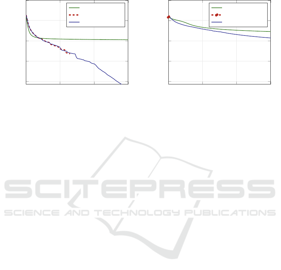
Figure 1 shows the attained loss measure deﬁned

in eq. (6) as it develops with equivalent epochs. The

genuine minimum is always zero. The plots corre-

spond to RMSprop in single precision as well as to

CG in single and double precision. The networks con-

sidered have one (ﬁg. 1a) and ﬁve (ﬁg. 1b) hidden lay-

ers.

Optimization results with shallow (single-hidden-

layer) neural networks have shown that the minimum

KDIR 2022 - 14th International Conference on Knowledge Discovery and Information Retrieval

310

0 2,000 4,000

6,000

−7

−5

−3

−1

Epoch Equivalent

Loss

RMSprop (single)

CG (single)

CG (double)

(a) One hidden layer (4mio-1h), moderate nonlinearity.

0 2,000 4,000

6,000

−7

−5

−3

−1

Epoch Equivalent

Loss

RMSprop (single)

CG (single)

CG (double)

(b) Five hidden layers (4mio-5h), moderate nonlinearity.

Figure 1: The largest one/ﬁve-hidden-layer networks (four million parameters) with moderate nonlinearity, loss progress (in

log scale) in dependence on the number of epochs.

MSE (known to be zero due to the task deﬁnitions)

can be reached with a considerable precision of 10

−6

to 10

−20

even for the largest networks. While double-

precision computation is not superior to single preci-

sion for smaller networks (in a range of one order of

magnitude), the improvements for the networks with

one and four million parameters are in the range of

two to six orders of magnitude. The optimization

progress for the largest network, comparing the de-

pendence on the number epoch equivalents for single

and double-precision arithmetic is shown in ﬁg. 1a.

With both precisions, CG exhibits superlinear

convergence property: between epochs 1,000 and

6,000, the logarithmic plot is approximately a straight

line. So every iteration leads to an approximately

ﬁxed multiplicative gain of precision of the minimum

actually reached. The single-precision computation,

however, stops after 2,583 epochs (156 iterations) be-

cause line search can’t ﬁnd a better result given the

low precision boundary. In other words, the line

search in single precision is less efﬁcient. This would

be an argument in favor of double precision.

For the network with a single hidden layer, the CG

algorithm is clearly superior to RMSprop. The largest

network attains a minimum error precision better by

ﬁve orders of magnitude, and possibly more when in-

creasing the number of epochs. The reason is the su-

perlinear convergence of CG obvious from (ﬁg. 1a).

It is interesting that in the initial phase, RMSprop

descends faster, quickly reaching the level that is no

longer improved in the following iterations.

However, with a growing number of hidden lay-

ers, the situation changes. For ﬁve hidden layers,

single-precision computations lag behind by two or-

ders of magnitude. The reason for this lag is different

from that observed with the single-hidden-layer tasks:

the single-precision run is prematurely stopped after

less than ﬁve CG iterations, because of no improve-

ment in the line search. This is why the line of the

loss for single-precision CG can hardly be discerned

in ﬁg. 1b. By contrast, the double-precision run pro-

ceeds until the epoch limit is reached (655 iterations).

As seen in ﬁg. 1b, the superlinear convergence

property with the double-precision computation is

satisﬁed at least segment-wise: a faster segment until

about 1,000 epoch equivalents and a slower segment

from epoch 4,000. Within each segment, the logarith-

mic plot is approximately a straight line. (Superlin-

earity would have to be rejected if the precision gain

factors would be successively slowing down, particu-

larly within the latter segment.)

For RMSprop, a lag behind the CG can be ob-

served with ﬁve hidden layers, but the advantage of

CG is minor — one order of magnitude. However, the

plot suggests that CG has more potential for further

improvement if provided additional resources. Once

more, RMSprop exhibits fast convergence in the ini-

tial optimization phase followed by weak improve-

ments.

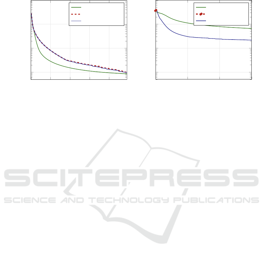
5.2 Strongly Nonlinear Problems

Mapping tasks generated with nonlinearity parameter

d = 4 imply strong nonlinearities in the sigmoid ac-

tivation functions with 5 % of activations having an

activation function derivative of less than 0.02. With

a linear term avoiding saturation (eq. (4)), this deriva-

tive grows to 0.07, a still very low value compared to

the unity derivative in the central region of the sig-

moid. The results are shown in ﬁg. 2 in the struc-

Training Neural Networks in Single vs. Double Precision

311

0 1,000 2,000 3,000 4,000

−2

−1

Epoch Equivalent

Loss

RMSprop (single)

CG (single)

CG (double)

(a) One hidden layer (4mio-1h), strong nonlinearity.

0 2,000 4,000

6,000

−2

−1

Epoch Equivalent

Loss

RMSprop (single)

CG (single)

CG (double)

(b) Five hidden layers (4mio-5h), strong nonlinearity.

Figure 2: The largest one/ﬁve-hidden-layer networks (four million parameters) with strong nonlinearity, loss progress (in log

scale) in dependence on the number of epochs.

ture analogical to ﬁg. 1. With CG, the parameter opti-

mization of networks of various sizes with one hidden

layer and two hidden layers shows no signiﬁcant dif-

ference between single and double-precision compu-

tations. The attainable accuracy of the minimum has

been, as expected, worse than for moderately nonlin-

ear tasks but still fairly good: almost 10

−5

for a single

hidden layer and 10

−2

for two hidden layers.

The relationship between both CG and RMSprop

is similar for single-hidden-layer networks (ﬁg. 2a)

— CG is clearly more efﬁcient. The attainable preci-

sion of error minimum is, as expected, worse than for

moderately nonlinear tasks.

For ﬁve hidden layers, a similar phenomenon as

for moderately nonlinear tasks can be observed: the

single-precision computation stops prematurely be-

cause line search fails to ﬁnd an improved value

(see ﬁg. 2b). The minimum reached is in the same

region as the initial solution.

The convergence of both algorithms (CG and

RMSprop) is not very different with ﬁve hidden layers

— superiority of CG is hardly signiﬁcant. Here, the

superlinear convergence of CG is questionable. The

reason for this may be a lack of convexity of the MSE

with multiple hidden layers and strongly nonlinear re-

lationships between input and output. It is important

to point out that the quality of the error minimum

found is extraordinarily poor: the MSE is about 10 %

of the output variance. This is 30 % in terms of stan-

dard deviation, which may be unacceptable for many

applications.

6 SUMMARY AND DISCUSSION

With the CG optimization algorithm, double preci-

sion computation is superior to single-precision in

two cases:

1. For tasks relatively close to convexity (single hid-

den layer networks with moderate nonlinearity),

the optimization progress with double-precision

seems to be faster due to a smaller number of

epochs necessary to reach a line search mini-

mum with a given tolerance. This allows the al-

gorithm to perform more CG iterations with the

same number of epochs. However, since both sin-

gle and double precision have the superlinear con-

vergence property, the gap can be bridged by al-

lowing slightly more iterations with single preci-

sion to reach a result equivalent to that of double

precision.

2. For difﬁcult tasks with multiple hidden layers

and strong nonlinearities, a more serious ﬂaw of

single-precision computation occurs: a premature

stop of the algorithm because of failing to ﬁnd

an objective function improvement by line search.

This may lead to unacceptable solutions.

In summary, it is advisable to use double precision

with the second-order methods.

The CG optimization algorithm (with double pre-

cision computation) is superior to the ﬁrst-order algo-

rithm RMSprop in the following cases:

1. Tasks with moderate nonlinearities. The advan-

tage of CG is large for shallow networks and less

pronounced for deeper ones. Superlinear conver-

KDIR 2022 - 14th International Conference on Knowledge Discovery and Information Retrieval

312

gence of CG seems to be retained also for the lat-

ter group.

2. Tasks with strong nonlinearities modeled by net-

works with a single hidden layer. Also here, su-

perlinear convergence of CG can be observed.

For tasks with strong nonlinearities and multiple hid-

den layers, both CG and RMSprop (which has been

by far the best converging method from those im-

plemented in the popular TensorFlow/Keras frame-

works) show very poor performance. This is docu-

mented by the square error attained, whose minimum

is known to be zero in our training examples. In prac-

tical terms, such tasks can be viewed as “unsolvable”

because the forecast error is too large in relation to the

output variability — the model gained does not really

explain the behavior of the output.

The advantage of RMSprop, if any, in some of the

strongly nonlinear cases is not very signiﬁcant (fac-

tors around two). By contrast, for tasks with either

moderate nonlinearity or shallow networks, the CG

method is superior. In these cases, the advantage of

CG is substantial (sometimes several orders of mag-

nitude). So in the typical case where the extent of

nonlinearity of the task is unknown, CG is the safe

choice.

It has to be pointed out that tasks with strong

nonlinearities in individual activation functions are,

strictly speaking, intractable by any local optimiza-

tion method. Strong nonlinearities sum up to strongly

non-monotonous mappings. But square errors of non-

monotonous mappings are certain to have multiple lo-

cal minima with separate attractors. For large net-

works of sizes common in today’s data science, the

number of such separate local minima is also large.

This reduces the chance of ﬁnding the global min-

imum to a practical impossibility, whichever opti-

mization algorithms are used. So the cases in which

the CG shows no signiﬁcant advantage are just those

“hopeless” tasks.

Next to the extent of nonlinearity, the depth of

the network is an important category where the alter-

native algorithms show different performances. The

overall impression that the advantage of the CG

method over RMSprop shrinks with the number of

hidden layers, that is, with the depth of the network,

may suggest the conjecture that it is not worth using

CG with necessarily double-precision arithmetic for

currently preferred deep networks (Heaton, 2018).

However, the argument has to be split into two dif-

ferent cases:

1. networks with fully connected layers

2. networks containing special layers, in particular

convolutional ones.

In the former case, the question is how far it is

useful to use multiple fully connected hidden layers at

all. Although there are theoretical hints that in some

special tasks, deep networks with fully connected lay-

ers may provide a more economical representation

than those with shallow architectures (Mont

ufar et al.,

2014) or (Delalleau and Bengio, 2011), the systematic

investigation of (Bermeitinger et al., 2019) has dis-

closed no usable representational advantage of deep

networks. In addition to it, deep networks are substan-

tially harder to train and thus exploit their representa-

tional potential. This can also be seen in the results

presented here. Networks with ﬁve hidden layers, al-

though known to have a zero error minimum, have not

been able to be trained to a square error of less than

10 % of the output variability. Expressed in standard

deviation, the standard deviation of the output error is

more than 30 % of the standard deviation of the output

itself. These 30 % do not correspond to noise inher-

ent to the task (whose error minimum is zero on the

training set) but to the error caused by the inability of

local optimization methods to ﬁnd a global optimum.

This is a rather poor forecast. In the case of the out-

put being a vector of class indicators, the probability

of frequently confusing the classes is high. In this

context, it has to be pointed out that no exact meth-

ods exist for ﬁnding a global optimum of nonconvex

tasks of sizes typical for data science with many lo-

cal minima. The global optimization of such tasks is

an NP-complete problem with solution time exponen-

tially growing with the number of parameters. This

documents the infeasibility of tasks with millions of

parameters.

Limitation to Fully Connected Networks. The

conjectures of the present work cannot be simply ex-

trapolated to networks containing convolutional lay-

ers — this investigation was concerned only with fully

connected networks. The reason for this scope limi-

tation is that it is difﬁcult to select a meaningful pro-

totype of a network with convolutional layers, even

more one with a known error minimum — the archi-

tectures with convolutional layers are too diversiﬁed

and application-speciﬁc. So the question is which op-

timization methods are appropriate for training deep

networks with multiple convolutional layers but a low

number of fully connected hidden layers (maybe a

single one). This question cannot be answered here,

but it may be conjectured that convolutional layers are

substantially easier to train than fully connected ones,

for two reasons:

1. Convolutional layers have only a low number of

parameters (capturing the dependence within a

small environment of a layer unit).

Training Neural Networks in Single vs. Double Precision

313

2. The gradient with regard to convolutional param-

eters tends to be substantially larger than that

of fully connected layers since it is a sum over

all unit environments within the convolutional

layer. In other words, convolutional parameters

are “reused” for all local environments that make

their gradient grow.

This suggests a meaningful further work: to ﬁnd

some sufﬁciently general prototypes of networks with

convolutional layers and to investigate the perfor-

mance of alternative optimization methods on them,

including the inﬂuence of machine precision for the

second-order methods.

REFERENCES

Bermeitinger, B., Hrycej, T., and Handschuh, S. (2019).

Representational Capacity of Deep Neural Networks:

A Computing Study. In Proceedings of the 11th Inter-

national Joint Conference on Knowledge Discovery,

Knowledge Engineering and Knowledge Management

- Volume 1: KDIR, pages 532–538, Vienna, Austria.

SCITEPRESS - Science and Technology Publications.

Chollet, F. et al. (2015). Keras.

Delalleau, O. and Bengio, Y. (2011). Shallow vs. Deep

Sum-Product Networks. In Advances in Neural Infor-

mation Processing Systems, volume 24. Curran Asso-

ciates, Inc.

Fletcher, R. and Reeves, C. M. (1964). Function minimiza-

tion by conjugate gradients. The Computer Journal,

7(2):149–154.

George, T., Laurent, C., Bouthillier, X., Ballas, N., and Vin-

cent, P. (2021). Fast Approximate Natural Gradient

Descent in a Kronecker-factored Eigenbasis.

Heaton, J. (2018). Ian Goodfellow, Yoshua Bengio, and

Aaron Courville: Deep learning. Genet Program

Evolvable Mach, 19(1):305–307.

Hinton, G. (2012). Neural Networks for Machine Learning.

Martens, J. (2010). Deep learning via Hessian-free opti-

mization. In Proceedings of the 27th International

Conference on International Conference on Machine

Learning, ICML’10, pages 735–742, Madison, WI,

USA. Omnipress.

Martens, J. and Grosse, R. (2015). Optimizing Neural Net-

works with Kronecker-factored Approximate Curva-

ture.

Mont

ufar, G. F., Pascanu, R., Cho, K., and Bengio, Y.

(2014). On the Number of Linear Regions of Deep

Neural Networks. In Ghahramani, Z., Welling, M.,

Cortes, C., Lawrence, N. D., and Weinberger, K. Q.,

editors, Advances in Neural Information Processing

Systems 27, pages 2924–2932. Curran Associates, Inc.

Nocedal, J. and Wright, S. J. (2006). Numerical Opti-

mization. Springer Series in Operations Research.

Springer, New York, 2nd ed edition.

Press, W. H., Teukolsky, S. A., Vetterling, W. T., and Flan-

nery, B. P. (1992). Numerical Recipes in C (2nd Ed.):

The Art of Scientiﬁc Computing. Cambridge Univer-

sity Press, USA.

Ren, Y., Bahamou, A., and Goldfarb, D. (2022). Kronecker-

factored Quasi-Newton Methods for Deep Learning.

TensorFlow Developers (2022). TensorFlow. Zenodo.

Virtanen, P., Gommers, R., Oliphant, T. E., Haberland, M.,

Reddy, T., Cournapeau, D., Burovski, E., Peterson, P.,

Weckesser, W., Bright, J., van der Walt, S. J., Brett,

M., Wilson, J., Millman, K. J., Mayorov, N., Nel-

son, A. R. J., Jones, E., Kern, R., Larson, E., Carey,

C. J., Polat,

I., Feng, Y., Moore, E. W., VanderPlas,

J., Laxalde, D., Perktold, J., Cimrman, R., Henriksen,

I., Quintero, E. A., Harris, C. R., Archibald, A. M.,

Ribeiro, A. H., Pedregosa, F., van Mulbregt, P., and

SciPy 1.0 Contributors (2020). SciPy 1.0: Fundamen-

tal algorithms for scientiﬁc computing in python. Na-

ture Methods, 17:261–272.

Wolfe, P. (1969). Convergence Conditions for Ascent Meth-

ods. SIAM Rev., 11(2):226–235.

KDIR 2022 - 14th International Conference on Knowledge Discovery and Information Retrieval

314