Mathematical Modeling of Morphogenesis and Population Dynamics
of Bacteria-Destructors during the Ellimination of Oil Pollution
A. I. Dzhangarov
1a
, N. V. Potapova
2
and R. U. Selimov
2
1
Kadyrov Chechen State University, 32 Sheripova Street, Grozny, Russia
2
Kuban State University, Krasnodar, Russia
Keywords: Software, mathematical models, morphogenesis, bacteria, oil pollution.
Abstract: In this scientific work, the process of constructing a mathematical model of morphogenesis and dynamics of
the number of bacteria that clean up oil pollution is considered. The creation of the model and the dedicated
accompanying software are extremely important in such studies. Automation of processes makes it possible
to predict the expected results and use various mathematical conditions and models in practice, in the field of
oil pollution.
1 INTRODUCTION
Preparation of Software. The software for
visualizing the mathematical model of the
morphogenetic development of the studied
microorganisms was developed using the Qt Creator
integrated software development environment in C++
using the Qt library set (Blagodatsky, 1998).
The choice in favor of this development
environment is due to its cross-platform nature - the
ability to create software that is compatible with
various operating systems (Windows, Linux, macOS,
Android, etc.), the rich functionality of the built-in set
of libraries and the wide possibilities in the field of
software rendering. Thus, it is possible to launch the
created software package on a wide range of
computer devices.
Such a feature of Qt as the use of APIs
(Application Programming Interface) of the low-level
operating system was also taken into account, which
makes it possible for the software created with it to
work as efficiently as the software that was developed
for specific platforms by other development tools
(Dalgaard, 2011).
An important factor in choosing a development
environment is the ability to quickly develop a user
interface. This is possible thanks to the Qt Designer
visual interface editing tool integrated into Qt Creator
(Pepper, 1995).
a
https://orcid.org/0000-0001-6962-9593
Study Materials. Cells of the strain A. globiformis
AC1112 pass through two stages in their
morphogenetic cycle of development: bacillus-
coccus (Hesty, 2017). During the lag phase, which
occurs approximately in the interval of 0-9 hours, the
cells increase in size (cocci with a diameter of 0.6 to
0.8 μm; rod-shaped from 2.3 × 0.5 to 3.1 × 0.7 μm ),
gradually transforming from coccoid to rod-shaped
forms, at the end of this stage, the appearance of V-
shaped and branched forms can also be observed. In
the exponential growth phase, which runs from 9 to
48 hours, cells, intensively dividing, decrease in size
(branched forms from 5.0 × 3.2 μm to 4.6 × 2.9 μm,
curved forms from 2.1 × 1 .0 to 2.1×0.7 µm) and show
different branching. The stationary phase occurs at
approximately 60 hours of cultivation. In this phase,
the branched forms, breaking up, give the original
coccoid forms, while the diameter of the emerging
cocci continues to be approximately 0.9 microns
(Linos, 2000).
Cells of the G. alkanivorans K9 strain in the lag
phase (0-12 h) are coccoid; here the cells slightly
increase in size (diameter from 0.5 to 1.1 microns). In
the exponential phase (12-60 hours), as the cultures
grow, the cells gradually transform into rod-shaped
cells, intensively divide, which leads to a decrease in
their size (rods - 2.3 × 0.9-1.6 × 0.6 μm) . Various
branches are observed here, as well as V-shapes,
curved forms (branched forms - 3.4 × 0.6-3.2 × 0.5
μm, curved forms - 2.1 × 0.7-2.0 × 0 .6 µm).
268
Dzhangarov, A., Potapova, N. and Selimov, R.
Mathematical Modeling of Morphogenesis and Population Dynamics of Bacteria-destructors during the Ellimination of Oil Pollution.
DOI: 10.5220/0011570100003524
In Proceedings of the 1st International Conference on Methods, Models, Technologies for Sustainable Development (MMTGE 2022) - Agroclimatic Projects and Carbon Neutrality, pages
268-273
ISBN: 978-989-758-608-8
Copyright
c
 2023 by SCITEPRESS – Science and Technology Publications, Lda. Under CC license (CC BY-NC-ND 4.0)

Subsequently, in the course of reaching the stationary
phase (about the 60th hour), the cells begin the
reverse transformation of cells of various forms into
the form of cocci.
2 MATERIALS AND METHODS
Establishing Correspondence between Real and
Theoretical Cell Shapes. For the most realistic
reflection of the morphology of microorganism cells
by the software package, a method was used, which
consists in the selection of proportionality
coefficients between different parts of the cell or the
entire cell, taking into account the experimental data
on cell sizes (Appendix A, tables A.3-A.4) obtained
in the course of the study. The location of the cells on
the field and the relative position of the parts of the
cell for complex (branched) forms in the software
package occurs randomly (Kummer, 2019).
Correspondence of real and theoretical forms of
cells created by means of the software package is
shown in Figures 1-2 for A. globiformis and Figures
3-4 for G. alkanivorans.
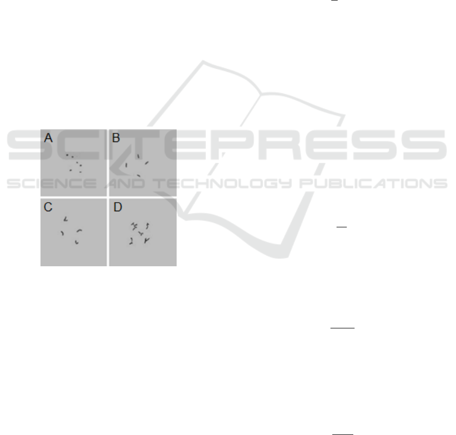
Figure 1: Natural forms of A. globiformis cells.
A - coccoid forms; B - rod-shaped forms; C -
curved and V-shape; D - branched forms.
Description of the Mathematical Model. t is the life
time of bacteria, determined by the formula (1):
,tHi=×
(1)
where t is the lifetime of bacteria, h; H is the
duration of the measurement period, h; i is the serial
number of measurements in the experiment.
In this study, the value of H is a constant and equal
to 3, the variable t varies between 0 and 44 (45
measurements in total), in accordance with the
number of experimental measurements. At
0t >
, the
process of growth of microorganisms begins, and
morphological changes in cells are observed
(Ordoñez, 2021).
L is the cell length. W is the cell width. V is the
volume of the cell: for cocci it is calculated according
to the standard formula for finding the volume of a
ball (formula (2)), and for rod-shaped ones, the
formula for the volume of a cylinder is used (formula
(3)), where the length of the cell L acts as the height,
and for complex forms (branched , V-shaped), the
volumes of individual rod-shaped branches are
summed up (formula (4)). The radius for all types of
cells (or their branches), except for cocci, is
determined by formula (5).
3
4
,
3
S
VR π =
(2)
where
S
V
is the volume of the coccoid cell,
3
мкм
; R is the cell radius, мкм .
2
,
С
VRL π =
(3)
where
С
V
is the volume of a rod-shaped cell,
3
мкм
; R is the cell radius, мкм ; L is the cell length,
мкм .
,
M
p
VV=

(4)
where
M
V
is the volume of complex-shaped cell,
3
мкм
;
P
V
is the volume of the rod-shaped branch of
a complex-shaped cell,
3
мкм
.
,
2
W
R =
(5)
where R is the cell radius,
мкм
; W is the cell
width,
мкм .
At each stage of morphogenesis, the average total
number of cells N was calculated in ten fields of view
(formula (6)):
,
10
i
N
N =

(6)
where N is the average total number of cells;
i
N
is the total number of cells in one field of view.
In the same way, for ten fields of view, the
average number of cells of individual forms
x
n
was
calculated (formula (7)):
,
10
i
x
n
n =

(7)
Mathematical Modeling of Morphogenesis and Population Dynamics of Bacteria-destructors during the Ellimination of Oil Pollution
269

where
x
n
is the number of cells of a given form;
i
n
is the number of cells of a given shape in one field
of view.
The quantitative proportion of cells of this form is
determined according to the formula (8):
,
x
x
n
v
N
=
(8)
where
x
v
is the quantitative proportion of cells of
a given form, %; N is the average total number of cells
in the field of view;
x
n
is the average number of cells
of a given shape in the field of view.
The volume fraction of cells of this form is
calculated by the formula (9):
,
x
x
i
v
V
ϕ =

(9)
where
x
ϕ
is the volume fraction of cells of a
given shape, %;
x
V
is the volume of a cell of a given
shape,
3
мкм
;
i
V
is the volume of a cell of a separate
form in a series,
3
мкм
.
The coefficient
x
L
, which reflects the volumetric
and quantitative ratio between individual cell forms,
is determined by formula (10):
,
ii
x
ii
v
L
v
ϕ
ϕ
=

(10)
where
x
L
is the linking coefficient;
x
v
is the
quantitative fraction of a cell of a given shape, %;
x
v
is the quantitative proportion of cells of individual
forms in the series, %;
x
ϕ
is the volume fraction of
cells of a given form, %;
i
ϕ
is the volume fraction of
cells of individual forms in the series, %.
The value
x
d
has been introduced, which links
the dynamics of changes in the process of growth and
development, both quantitatively and qualitatively -
this is an indicator of the partial optical density for
cells of a certain shape at a point in time. It is
calculated for each type of cell shape individually.
This value is determined by formula (11):
,
x
ix
dDL=
(11)
where
x
d
is the partial optical density;
i
D
is the
optical density of cell culture at this stage;
x
L
is the
linking coefficient.
Based on the principle of optical density
additivity, the unknown optical density of the cell
culture D can be calculated by adding the known
partial optical densities (formula (12)).
,
i
Dd=

(12)
where D is the optical density of the cell culture;
i
d
is the partial optical density of cells of individual
forms.
Having data on the initial values of the number of
cells
0
N
and the optical density of the cell culture
0
D
, it is possible to calculate the number of cells at a
given stage of growth for a given form of cells at a
given stage of morphogenesis (formula (13)).
0
0
,
x
x
ND
n
LD
=
(13)
where
x
n
is the number of cells of a given form;
0
D
is the initial optical density of the cell culture; D
is the optical density of cell culture at this stage.
In the same way, the total number of cells is the
sum of the number of individual cell shapes (formula
(14)), known in advance or calculated using the above
computational model constructs.
,
i
Nn=

(14)
where N is the total number of cells;
i
n
is the
number of cells of individual forms.
Determination of the Dependence of the Rate
of the Course of the Morphogenetic Cycle of
Development of Microorganisms on the
Temperature of the Environment.
In the
framework of studies on the development of
microorganisms, it often becomes necessary to
establish the dependence of the growth rate on
temperature. In modeling the processes of growth and
development of bacterial cells, the equations of linear
dependence have proven themselves very
successfully. Here, the function y=k(T) is used, where
k is an absolute indicator that characterizes growth at
a certain temperature of the medium. In most cases, it
is calculated from the initial and final number of cells;
however, in this work, instead of these parameters, we
resorted to using the initial and final optical density
(formula (15)). The determining value in equations of
this type is the angular coefficient of the straight line,
which characterizes the dynamics of the change in the
value of k under different temperature conditions of
growth.
,
i
Nn=

(15)
MMTGE 2022 - I International Conference "Methods, models, technologies for sustainable development: agroclimatic projects and carbon
neutrality", Kadyrov Chechen State University Chechen Republic, Grozny, st. Sher
270

where k(T) is the absolute dependence of the MO
growth rate on temperature, h-1; Dt is the final OD of
cells; D0 is the initial OD of cells; tp is the duration
of the logarithmic stage of growth, h.
The optimal temperature limits for growth for
many coryneform bacteria are 20–30 degrees Celsius,
so only these limits were considered in this work.
Since the most detailed morphological studies and
related calculations were carried out at 30 °C, it is
necessary to ensure that the value of the parameter k
at a value of T = 30 °C is equal to one. To do this, we
introduced a correction factor a (it has a unique
numerical value for each microorganism), which will
allow us to correct the model parameters taking into
account the available experimental data, and obtained
a computational design for calculating another
parameter - the relative dependence of the growth rate
of microorganisms on temperature - r(T) (formula
(16)):
() (),rT a kT=×
(16)
where
()rT
is the relative dependence of the MO
growth rate on temperature,
1
r
−
; a is the correction
factor;
()kT
is an indicator of the absolute
dependence of the
MO growth rate on temperature,
1
r
−
.
Calculation of Appropriate Models for
Morphogenesis. Based on the experimental data
obtained from the study of cells of bacterial strains,
graphs were plotted, where the cultivation time was
plotted on the abscissa axis, and the optical density
was plotted on the ordinate axis, and growth curves
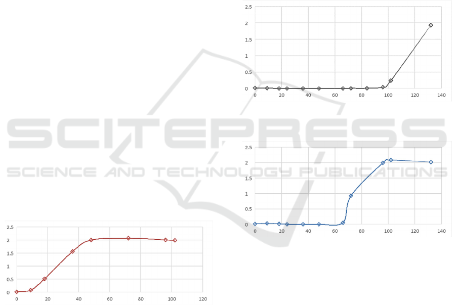
were obtained (Figure 2).
Figure 2: Globiformis growth curve at 30 °C.
In order to assess the contribution of cells of
various shapes to the optical density, i.e., to calculate
the partial optical density
d, it was necessary to
perform some intermediate calculations, namely:
based on data on cell sizes, determine the volumes
occupied by cells
V (according to formulas (2) - (4)),
volume fractions
x
ϕ (according to formula (9)).
Having obtained the values of cell volumes
V and
then their volume fractions
x
ϕ , and having known
percentages of various cell shapes
x
v , it is possible
to determine the coefficient
x
L by formula (10), and
subsequently, according to formula (11), the partial
optical density
x
d for strain A (globiformis).
Similarly, the corresponding values of the partial
optical density
x
d were calculated for strain G.
(alkanivorans K9).
At the next stage, the obtained data were used to
plot graphs that reflect the patterns of changes in cell
morphology in the morphogenetic cycle of
development of the studied bacterial strains, taking
into account their contribution to the readings of
optical density (Figures 3-4).
Figure 3: Dynamics of changes in partial optical density
coccoid cell forms for A (globiformis, at 30°C).
Figure 4: Dynamics of changes in partial optical density
coccoid cell forms for G (alkanivorans, at 30°C).
For the convenience of work, the obtained graphs
of the curve of the dynamics of changes in the partial
optical density
x
d for each culture, in turn, were
divided into several time intervals (Perni, 2005). In
addition to convenience, this was done to avoid
overcomplicating features. And, based on their
belonging to a certain type of charts, with the help of
Microsoft Excel, a trend line and the corresponding
approximating function were selected. In this case,
the zero values of the functions were taken out of the
graph, taking into account separately. The reliability
coefficients for the approximation of
2
R
functions
have been brought to values as close as possible to
unity in order to most accurately reflect the dynamics
Mathematical Modeling of Morphogenesis and Population Dynamics of Bacteria-destructors during the Ellimination of Oil Pollution
271

of the described processes. Figures 4-6 show the
intervals of the graph for coccoid forms of culture
A
(globiformis) with approximated functions, which
subsequently become functions of the mathematical
model, and calculated confidence factors.
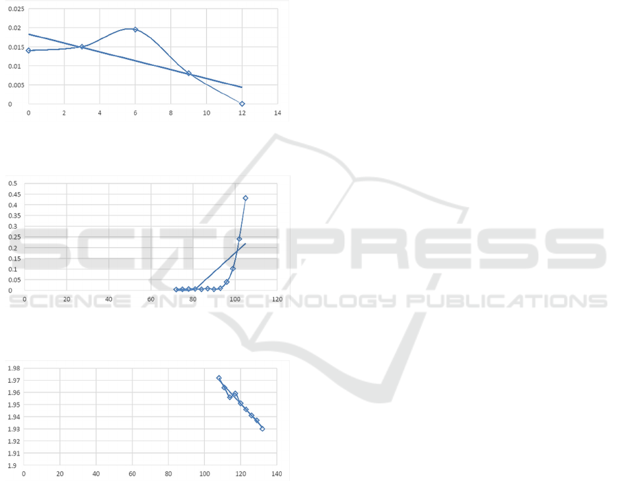
Thus, the curve of the dynamics of changes in the
partial optical density
d(t) of culture A (globiformis)
for coccoid forms is divided into segments 0-12, 72-
105 and 108-132 hours (Figures 5-7). The first two
curves are described by a polynomial type trend line,
the last one by a linear type.
Figure 5: Curve and trend line for coccoid cell shapes A
(globiformis between 0-12 hours, at 30°C).
Figure 6: Curve and trend line for coccoid forms A
(globiformis cells within 72-105 hours, at 30°C).
Figure 7: Curve and trend line for coccoid cells of A
(globiformis between 108-132 hours, at 30°C).
3 RESULTS AND DISCUSSION
As a result, by combining individual functions into a
system, taking into account the zeros of the functions,
an equation of the model for the morphogenesis of
microorganisms was obtained for the mathematical
model developed within the framework of this study.
Culture A (globiformis) corresponds to formula:
422
( ) {0,0002 0,00048 0,00326 0,00565 }
[0; 132]
dttttt
t
=−+ −
∈
where
t is the lifetime of bacteria.
Thus, the growth of microorganisms depends on
their life cycle, and the longer it is, the higher their
efficiency in the treatment of oil pollution. In
addition, it should be noted that additional factors
affecting their effectiveness in terms of cleaning can
be such parameters as temperature, pressure and
stimulants, inhibitors, and so on. The construction of
a mathematical model is very significant, since it
allows the use of various software systems, which
were discussed earlier (Magomedov, 2022). There are
special libraries in the C++ programming language
that have built-in methods for working with
mathematical models and their visualization. Such a
solution is also intended to speed up laboratory
research, which can sometimes take a long time.
4 CONCLUSIONS
In conclusion, we can say that the morphogenetic
development of A. globiformis AC1112 and G.
alkanivorans K9 strains was studied: they are
represented by the bacillus-coccus cycle and growth
curves characterizing the increase in cell biomass
(Moussa, 2020).
The physical dimensions of the cells during their
growth, the diameter of A. globiformis cocci and G.
alkanivorans cocci were determined; sizes of rod-
shaped, branched-shaped, curved and V-shaped. The
dependence of the growth of microorganisms on the
temperature conditions of cultivation, the content of
biogenic elements in the oil sludge medium and their
relationship with other parameters of the processes
under study has been established.
A mathematical model of morphogenesis and
population dynamics of A. globiformis and G.
alkanivorans in the process of oil pollution clean-up
has been created. On its basis, software was
considered and tested that allows determining the
growth stage based on input data on the temperature
of the cultivation medium and the content of biogenic
elements in oil sludge, as well as visualizing the
morphology of microorganisms. The model can serve
as a tool for optimizing the temperature and chemical
parameters of the growth environment of oil
degrading bacteria, as well as increasing the
efficiency of control during biological treatment.
MMTGE 2022 - I International Conference "Methods, models, technologies for sustainable development: agroclimatic projects and carbon
neutrality", Kadyrov Chechen State University Chechen Republic, Grozny, st. Sher
272

REFERENCES
Linos, A., 2000. Biodegradation of cis-1,4-polyisoprene
rubbers by distinct actinomycetes: microbial
strategies and detailed surface analysis. Appl.
Environ. Microbiol. 66. pp. 1639-1645.
Blagodatsky, S. A., Richter, O., 1998. Microbial growth in
soil and nitrogen turnover : a theoretical model
considering the activity state of microorganisms. Soil
Biology and Biochemistry. 30(13). pp. 1743-1755.
Hesty, H., Meilana, D. P., 2017. Kinetic study and
modeling of biosurfactant production using Bacillus
sp. Electronic Journal of Biotechnology. 27. pp. 49–
54.
Dalgaard, P., Koutsoumanis, K., 2011. Comparison of
maximum specific growth rates and lag times
estimated from absorbance and viable count data by
different mathematical models. Journal of
Microbiological Methods. 43(3). pp. 183–196.
Kummer, C., Schumann, P., Stackebrandt, E., 2019.
Gordonia alkanivorans sp. nov., isolated from tar-
contaminated soil. Int. J. Syst. Bacteriol. 49. pp. 1513-
1522.
Moussa, T. A. A., Ahmed, G. M., Abdel-Hamid, S. M.-S.,
2020. Mathematical model for biomass yield and
biosurfactant production by Nocardia amarae. New
aspects of fluid mechanics, heat transfer and
environment. pp. 27-32.
Perni, S., Andrew, P., Shama, W. G., 2005. Estimating the
maximum growth rate from microbial growth curves
: definition is everything. Food Microbiology. 22(6).
pp. 491–495.
Pepper, Ian, Gerba, Charles, Brendecke, Jeffrey, 1995.
Environmental Microbiology. A Laboratory Manual.
1st Edition.
Ordoñez, M., et. al., 2021. Propuesta metodológica para el
diseño de prótesis utilizando CAD generativo y
análisis CAE. p. 7.
Magomedov, I. A., Ordoñez-Avila, José Luis, Bagov, A. M.
2022. Statistical evaluation of a robotic six-wheel
structures mechanism based on motion simulation.
Mathematical Modeling of Morphogenesis and Population Dynamics of Bacteria-destructors during the Ellimination of Oil Pollution
273