ECD Test: An Empirical Way based on the Cumulative Distributions to

Evaluate the Number of Clusters for Unsupervised Clustering

Dylan Molini

and Kurosh Madani

LISSI Laboratory EA 3956, Universit

e Paris-Est Cr

eteil, S

enart-FB Institute of Technology,

Campus de S

enart, 36-37 Rue Georges Charpak, F-77567 Lieusaint, France

Keywords:

Unsupervised Clustering, Parameter Estimation, Cumulative Distributions, Industry 4.0, Cognitive Systems.

Abstract:

Unsupervised clustering consists in blindly gathering unknown data into compact and homogeneous groups; it

is one of the very ﬁrst steps of any Machine Learning approach, whether it is about Data Mining, Knowledge

Extraction, Anomaly Detection or System Modeling. Unfortunately, unsupervised clustering suffers from the

major drawback of requiring manual parameters to perform accurately; one of them is the expected number

of clusters. This parameter often determines whether the clusters will relevantly represent the system or not.

From literature, there is no universal fashion to estimate this value; in this paper, we address this problem

through a novel approach. To do so, we rely on a unique, blind clustering, then we characterize the so-

built clusters by their Empirical Cumulative Distributions that we compare to one another using the Modiﬁed

Hausdorff Distance, and we ﬁnally regroup the clusters by Region Growing, driven by these characteristics.

This allows to rebuild the feature space’s regions: the number of expected clusters is the number of regions

found. We apply this methodology to both academic and real industrial data, and show that it provides very

good estimates of the number of clusters, no matter the dataset’s complexity nor the clustering method used.

1 INTRODUCTION

In the area of Machine Learning, clustering is a ma-

jor cornerstone: it is often used to preprocess data,

or to highlight hidden information. Maybe one of the

most interesting applications of clustering is the auto-

matic labeling of data, which allows the use of super-

vised (learning) methods downstream – the automatic

labeling performed by unsupervised clustering aims

to replace a manual labeling (Molini

e et al., 2021).

Although promising, clustering has some limits.

The ﬁrst is the accuracy of the results: since we deal

with blind methods, it is very hard to state on the ac-

curacy – and on the relevance alike – of the obtained

clusters. To handle that, we proposed BSOM, a two-

level clustering method based on the averaging of sev-

eral clusterings, so as to diminish the scattering of

the results whilst maximizing the number of scenar-

ios taken into account (Molini

e and Madani, 2022).

The second limitation of clustering is related to

the meta-parameters. Actually, alike most unsuper-

vised approaches, some parameters must be set man-

ually, which greatly impacts the results, especially

in a blind, unsupervised context. As a consequence,

https://orcid.org/0000-0002-6499-3959

the parameters should be chosen very wisely; but the

question remains quite simple: how to do so?

Indeed, the true reason for using unsupervised

learning is that one needs no previous information on

the data; ironically, the meta-parameters are the para-

dox of unsupervised learning, for they require some

speciﬁc knowledge to be set correctly. Even though

every method has its own meta-parameters, there is

one required by most of them: the (expected) number

of clusters; for instance, it is the K of the K-Means,

or the grid’s size of the Self-Organizing Maps. This

parameter is incontestably the most sensitive one, for

it may change the results in depth. Note that some

methods do not need this parameter, such as hierarchi-

cal approaches (e.g., Ascending Hierarchical Classiﬁ-

cation, Tree-like Divide To Simplify); however, they

suffer from another drawback with their thresholds

and split criteria (when to isolate data from others).

As a consequence, ﬁnding a way to estimate the

optimal value to set the meta-parameters to – and es-

pecially the number of clusters – becomes crucial,

even though there exists no such tool. A piece of so-

lution may come along an upstream analysis of the

database before processing; for instance, one may

study the relation between data in order to see if any

Molinié, D. and Madani, K.

ECD Test: An Empirical Way based on the Cumulative Distributions to Evaluate the Number of Clusters for Unsupervised Clustering.

DOI: 10.5220/0011562500003329

In Proceedings of the 3rd International Conference on Innovative Intelligent Industrial Production and Logistics (IN4PL 2022), pages 279-290

ISBN: 978-989-758-612-5; ISSN: 2184-9285

279

redundancies appear, which could drive the choice of

the number of clusters. Unfortunately, attempting to

ﬁnd a universal characteristic suitable to any database

is just a waste of effort (Molini

e et al., 2022).

In this paper, we address that actual problem,

through an empirical fashion. Indeed, whilst it is very

hard to ﬁnd a universal criterion to any database, noth-

ing prevents from applying a ﬁrst, raw clustering, at a

ﬁne grain for instance, and then reﬁne it further, and

eventually use the reﬁned version of the clustering as

an indicator of a good candidate for the number of

clusters. Note that reﬁning a database such way and

proceeding to a clustering with a good value for the

number of clusters are two different things, since re-

doing a clustering with the correct meta-parameters

takes beneﬁt from the intrinsic ability of the clustering

method for data organization, i.e., the learning step,

which is lost when only reﬁning the clusters.

First, we will begin with a short overview of some

already-existing methods to evaluate the number of

clusters, and we will move on to the detailed descrip-

tion of the proposed method. Then, we will assess

this technique with both academic and real industrial

data, and we will eventually conclude this paper.

2 STATE-OF-THE-ART

There exists two ways of evaluating the optimal pa-

rameters of an algorithm: 1- By a deep upstream anal-

ysis, based on heavy mathematical tools; 2- Through

an empirical approach based on the example. The for-

mer has the advantage of leading to more accurate re-

sults (mathematically ”optimal”), but has the major

drawback of being very heavy to perform, and lowly

generalizable (which tool to use?); on the contrary,

the latter has the advantage of being easier and more

universal, but has the limitation of achieving less ac-

curate results (empirically adapted, but not optimal)

Unfortunately, thus far, no mathematically opti-

mal solution has been proposed to the problem of de-

termining the number of clusters of a dataset; one gen-

erally has to content oneself with heuristics, i.e., ac-

ceptable estimates with respect to the observed data.

These heuristics can be gathered into two groups:

1- The theoretical ones, which apply some tools to the

database so as to estimate the empirically ”optimal”

number of clusters; 2- The true empirical ones, which

simply cluster the database several times by varying

This limitation is not a real one in Physics and Ma-

chine Learning, for an optimized solution is generally well-

suited for models, but often not applicable to real situations.

Moreover, an experimental dataset can differ from a record

to another, thus the optimal solution may vary between both.

the value of the number of clusters, and eventually

select the clustering (and thus the number of clusters)

which minimizes any criterion. Most of the methods

of the literature belong to the second category.

From the rare methods of the ﬁrst category, it is

worth mentioning (Honarkhah and Caers, 2010). The

authors assumed that any dataset can be linearly clus-

tered in an appropriate space, called kernel space

; to

do so, one must have recourse to a dedicated transition

matrix, called kernel matrix, which projects the data

from the original space to the kernel space. The au-

thors suggested that this matrix would contain much

information, and especially that plotting its eigenval-

ues, sorted and weighted by the normalized dot prod-

uct of their eigenvectors, would lead to a good esti-

mate of the number of clusters as of the curve’s knee.

They got good results on simple examples, but this

method suffers from two major drawbacks: ﬁrstly,

the projection into the kernel space is a complex and

time-consuming operation; secondly, the kernel to use

must be deﬁned manually upstream, which requires

some kind of knowledge (such as the possible data’s

distribution), and thus we are replacing a knowledge

(the number of clusters) by another (the kernel).

Otherwise, some methods rely on the Akaike or

the Bayesian Information Criteria (AIC and BIC, re-

spectively (Goutte et al., 2001; Pelleg and Moore,

2002). Based on a pure statistical estimation of the

information contained within a dataset, these criteria

can be used in some fashion so as to provide an esti-

mate of the number of clusters. Nonetheless they are

generally used as simple indicators of clustering qual-

ity in an empirical fashion by running the clustering

several times, incrementing each time the number of

clusters, and by eventually selecting the value maxi-

mizing these information criteria.

On the opposite, the second category’s methods

operate much simpler: they cluster the data with dif-

ferent values for the number of clusters, compute

some quality criteria, and eventually select that with

the best results. Notice that even though these tech-

niques claim that they are able to ﬁnd a good candi-

date for the number of clusters, they are actually not

sensu stricto; indeed, they actually think and operate

the other way round: the interest in ﬁnding a good

candidate for the number of clusters is precisely to

obtain a good clustering, but there is no need for this

parameter if one already has the best results just by

chance or by brute force. These methods are more an

empirical way to ﬁnd the best clustered version of a

database rather than a true way to estimate the optimal

number of clusters.

For instance, two circles can be linearly separated if

the space is circular, since a line in this space is a true circle.

ETCIIM 2022 - International Workshop on Emerging Trends and Case-Studies in Industry 4.0 and Intelligent Manufacturing

280

That being said, they propose some variations, and

especially a quantiﬁcation of the information brought

by the addition of new clusters; indeed, very likely

when adding new clusters, they should be more com-

pact, and thus should carry more information, but

there is often a point from which adding new clusters

is not really useful. For instance, consider a database

with 5 classes: clustering it with 5 clusters should be

the best option, but using 10 clusters will probably

lead to more compact groups, thus the quality of that

last clustering will be better. Most techniques from

the literature aim to address that problem of informa-

tion, by proposing an empirical trade-off: which value

to use to get the most information, while also not de-

grading the clustering relevance too much?

This is for instance the Elbow method’s purpose

(Marutho et al., 2018): it plots the explained vari-

ance against the number of clusters, and selects as

best candidate (trade-off) for the number of clusters

the curve’s knee (also called elbow). Simple method,

it can provide a correct estimate, but there is no certi-

tude that such inﬂection point actually exists.

Similarly, instead of using the explained variance,

(Amorim and Hennig, 2015) proposed to use the Sil-

houette Coefﬁcients, a compactness quantiﬁer pop-

ular in clustering (Rousseeuw, 1987), while keeping

the same methodology, i.e., plotting the mean Silhou-

ettes against the number of clusters, and eventually

return the curve’s knee. These coefﬁcients are highly

representative of the quality of the clustering (Molini

et al., 2022), but are very long to compute: the method

is slightly more representative, but longer to perform.

A last work to mention may be (Tibshirani et al.,

2001), which processes the same way than the two

previous methods, but this time replacing the metrics

by the explained variation, i.e., the part of the ob-

served variance in the theoretical variance of a model.

To do so, the idea is to build a ”ground truth” model

under the null hypothesis, i.e., with the same charac-

teristics (particularly the mean and variance) than the

database, cluster it several times and ﬁnally compare

how close to the clustering performed over the real

data it is. This procedure is repeated with several val-

ues set for the number of clusters, and that obtaining

the less dissimilarity between the clustered ”ground

truth” and the real clustered database is chosen as the

best candidate. This method led to quite good results,

but requires a model to build the ground truth upon

and is incredibly complex for such a simple purpose.

As a summary, there are two ways to estimate the

number of clusters: by a theoretical analysis or by

testing several values and selecting that minimizing

any criterion. In this paper, we propose a third kind

of methodology, halfway between both.

3 PROPOSED SOLUTION

The main problem with fully theoretical approaches is

that they are generally very complex, often too com-

plex for the user’s real purposes. Indeed, it is not rare

that a mathematically optimal solution to a physical

problem is not applicable as it is to real situations, due

to the intrinsic imperfections of the real system. An

optimal solution suits well simulations, but an only

approximated solution is often more than enough for

real systems. Of course, that is not always true, such

as in aviation or with critical systems for instance,

where an exact solution is absolutely necessary; but

where unsupervised learning can be used, such accu-

racy is generally not mandatory, whence the use of

empirical approaches can be justiﬁed.

Moreover, empirical methods have another great

advantage over theoretical ones: they perfectly suit

the observed data in a given context; they actually are

more practical and data oriented.

For these reasons, we have favored an empirical

approach for the estimation of the number of clusters

contained within a database. Nonetheless, we did not

want to propose another clustering method, which is

somehow what the Elbow method and assimilated do

in testing several clusterings and eventually selecting

that minimizing any criterion. As a consequence, we

thought about a different methodology which would

provide a true empirical value for the number of clus-

ters but without unnecessarily testing many.

In short, our methodology can be summarized as

follows: 1- Cluster the database only once, but with a

large number of clusters; 2- Characterize the clusters

in some fashion; 3- Regroup the clusters according

to the closeness of their characteristics computed in

the previous point; 4- Return the estimated number of

clusters as of the number of so-built ”super-groups”.

Remark that this is not a new clustering, but actu-

ally a true estimation of the number of clusters. So as

to get a true clustering method, we could have merged

repeatedly the clusters in a hierarchical fashion, but

that already exists and is entitled agglomerative clus-

tering (Sibson, 1973; Defays, 1977). Getting a good

estimate for the number of clusters aims to put every-

thing in place for the true Machine Learning cluster-

ing step thereafter. Indeed, the learning step would

be lost in the clusters merging, whilst setting the op-

timal parameters to the clustering method would take

advantage of all its abilities.

In all the following, we will refer to the real num-

ber of clusters as K, the estimated number as K

′

, the

database as D = {x

}

n∈[[1,N]]

with N = |D| the number

of data within, the clustering C = {C

}

k∈[[1,K]]

with C

the cluster k, and denote d as a distance.

ECD Test: An Empirical Way based on the Cumulative Distributions to Evaluate the Number of Clusters for Unsupervised Clustering

281

3.1 Clustering

In our methodology, the very ﬁrst step is clustering:

it consists in gathering data into compact and homo-

geneous groups, within which they share similarities,

while differing from a group to another. In practice,

most unsupervised clustering methods aim to mini-

mize the statistical ”error” between the clusters and

data. As an example, by considering that the distance

between a data and the barycenter of its correspond-

ing cluster is such an error, the total error of the clus-

tering is the sum of these local distances, for all the

data, for all the clusters: clustering aims to reduce this

sum. Actually, it is mostly a matter of optimization,

but hidden behind a dedicated formalism.

There exists plenty of clustering methods, either

supervised (SVM, Random Forests) or totally blind

(K-Means, SOMs). The choice of the method to use

depends on the context and on the objectives.

Supervised clustering consists in searching for

the best borders between different, already-labeled

classes, by adapting a shape (line, curve) to the space

between them; note that, here, the classes are known,

whence the use of ”class” instead of ”cluster”. Un-

supervised clustering consists in blindly regrouping

data into compact groups, with no previous assump-

tion on them; neither the barycenters of the classes,

nor even their number are known, whence the term

unsupervised. The former achieves better results,

but assumes much information on the data (their true

classes), whereas the latter is more universal, but the

quality and relevance of its output is not certain.

In an Industry 4.0 context, we study the relevance

of using Data Mining methods to dig into data, and

extract whatever knowledge can be found. As such,

we mainly rely on unsupervised learning, for we aim

to investigate highly generalizable works. For these

reasons, we will only present unsupervised clustering.

The ﬁrst to be introduced is the K-Means, the

reference clustering method (Lloyd, 1982): it draws

K points as barycenters, aggregates the surrounding

data around these points according to their respec-

tive closeness, and then updates the barycenters as

the true means of the so-built groups; this operation

is repeated a certain number of times or until satisfy-

ing any criterion. The K-Means is a very-well known

clustering algorithm, but also very naive and simple:

it has the major limitation of being able to separate

only linearly separable datasets, and therefore poorly

suitable for real situations such as industrial systems.

To compensate that, one may operate in a kernel

space, where the data would be ”linearly” separable,

provided that a line in such space is a nonlinear curve

in the original space. Once the data projected into this

nonlinear space, one may apply the K-Means to them;

this method is called Kernel K-Means (Dhillon et al.,

2004). Notice that this kernel version also exists for

many methods (Kernel SOM, SVM, etc.).

Better than the K-Means and more adapted to non-

linearly separable datasets, one may also consider

the Self-Organizing Maps (SOMs) (Kohonen, 1982);

they can be seen as a generalization of the K-Means

in which the learning step is nonlinear, and where the

different clusters are connected to each other within a

map, called a grid. This linkage aims to maintain the

topology of the database, while also accelerating the

learning by using a notion of neighborhood.

In (Molini

e et al., 2021), we tested the K-Means,

Kernel K-Means and SOMs on real industrial data,

and concluded that the last method is that which

works best, by providing the most representative clus-

ters, i.e., the closest to the real system’s behaviors.

In (Molini

e and Madani, 2022), we proposed an

improvement to the SOMs as of the Bi-Level Self-

Organizing Maps (BSOMs), a two-level clustering

aiming to reduce the scattering of the results, while

also improving their accuracy and relevance. In-

deed, alike any unsupervised method, the initializa-

tion should be random so as to avoid bias; but do-

ing so may scatter the results: there is no certitude

that two runs of the same algorithm give the same re-

sults. To compensate that, we proposed to build sev-

eral maps, with different initializations and learnings

(ﬁrst level), and eventually project all of them into a

ﬁnal map using the SOMs (second level), giving birth

to what we called BSOM. We tested it on real indus-

trial data anew, and, compared to the K-Means and to

the original SOMs, BSOM proved to be more accu-

rate, less volatile (more consistent results between the

runs) and closer to the real objective clusters, i.e., the

real behaviors of the industrial system we considered.

In this paper, we will use the K-Means, the SOMs

and BSOM to assess our methodology of determin-

ing the best candidate for the number of clusters, i.e.,

K for the ﬁrst, and the grid’s size for the two others.

Figure 1 gives an example of results for each method,

applied to a handful of Gaussian distributions; even

though it is pretty subjective, BSOM seems to give

the best clustering, with the most consistent regional

groups, then SOM and ﬁnally the K-Means.

3.2 Cumulative Distributions

Once the clusters built, they must be characterized;

this can be done in many fashions: feature vector,

compactness, homogeneity, etc. Some of these in-

dicators aim to measure the quality of the clusters,

i.e., how similar the data within are, and/or how far

ETCIIM 2022 - International Workshop on Emerging Trends and Case-Studies in Industry 4.0 and Intelligent Manufacturing

282

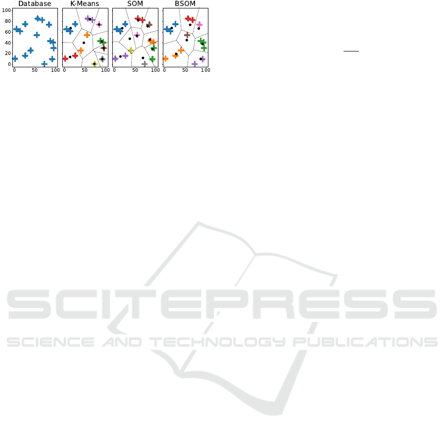
Figure 1: Example of clustering with different methods.

from the other clusters they are; this is for instance the

case with the Silhouette Coefﬁcients. On the contrary,

some of these quantiﬁers aim to describe the clusters,

i.e., propose a characteristic unique to them and al-

lowing to ﬁnd them back or compare them between

each other: this is for example the case with descrip-

tor vectors, which are commonly used in computer

vision so as to simplify the comparison of images, or

to search for the same object in different images.

In order to evaluate the quality of the clustering,

the ﬁrst category of methods is the most appropriate;

on the opposite, if the purpose is to compare the clus-

ters with each other, the second category of methods

should be considered ﬁrst. In our case, since we want

to estimate how similar the clusters are, so as to link

them in some fashion, the second category of methods

is the most appropriate for us.

Consequently, we are looking for a characteristic

unique to every cluster, which would indicate that two

clusters are very close (or distant) in the feature space,

but without necessarily taking account their inner

quality. To that purpose, the Average Standard Devia-

tion (Rybnik, 2004), the Hyper-Density (Molini

e and

Madani, 2021) or the Silhouettes (Rousseeuw, 1987)

would be of little help; in fact, we need more a char-

acteristic than a true compactness measure.

There exists thousands of tools to characterize (or

just compare) groups of data: mathematical moments

(mean, variance, etc.), intercluster distances, linkages

(single, complete, Ward, etc.), correlation, etc. Each

one of them has its own advantages and drawbacks:

for instance, correlation is only able to detect linear

similarity between groups of data; a linkage does not

necessarily take into account the outliers; and a statis-

tical moment can be routed by the physical proximity

of the clusters in the feature space.

As such, inspired by the Kolmogorov-Smirnov

(KS) Test (Simard and L’Ecuyer, 2011; Hassani and

Silva, 2015), we propose to use the Empirical Cumu-

lative Distributions (ECDs) of the clusters. Indeed,

they are highly representative of the clusters: they in-

dicate how the data within are distributed, with the

great advantage of considering the data’s intrinsic val-

ues, contrary to most of the metrics discussed earlier.

The ECD of a cluster represents the empirical

probability that its data are lower than a threshold; for

cluster C

, this probability P

is given by formula (1).

∀x ∈ R, P

(x) =

∑

∈C

≤x

(1)

with 1

≤x

the indicator function of {x

∈ R | x

≤ x},

and deﬁned by (2).

∀x

,x ∈ R, 1

≤x

(

1, if x

≤ x

0, else

(2)

Notice that one may derive function 1

≤x

from

the (delayed) Heaviside step function H, as of (3).

∀x

,x ∈ R, 1

≤x

= 1 − H(x

− x) (3)

Finally, the ECD of cluster C

is deﬁned as the set

of all the empirical probabilities, as of (4).

ECD



(x)



x∈R

(4)

Notice that the ECD should not be computed for

any real value, but only for that belonging to the do-

main of the database; in practice, this set is computed

for a ﬁnite number of x, ranging from the database’s

minimum to its maximum with a given step.

The ECDs are very useful to understand how the

data are distributed within a cluster. Moreover, since

they are based on absolute values, they also have a

physical meaning, related to achieved values; indeed,

if two datasets have close ECDs, it means that their

data distributions are close alike, both in compact-

ness and in absolute values. To keep it simple, the

slope of an ECD indicates the compactness (the larger

the slope, the more compact the data), whilst its posi-

tion indicates the position of the data within the space.

That last point is the core of our methodology, and the

main reason why we chose the ECDs over any other

metric: by comparing two of them, it is possible to de-

cide if two clusters are similar (density, compactness),

but also if they are just close in the space.

Notice that there is one ECD by dimension, which

must be fused in some fashion so as to provide a scalar

as of the number of clusters. One may think about tak-

ing their average, computed over all the dimensions,

but this could create false correspondence. For in-

stance, assuming x and y belong to the same interval I,

the function f

(x,y) = x and the function f

(x,y) = y

are very different, but have the same mean over the

two dimensions. This is a good example of the limit

of averaging; to avoid such case, we propose to state

that two distributions are very close if that is true for

all the dimensions at the same time.

As an example, Figure 2 depicts the ECDs of both

dimensions of the clusters given by BSOM (rightmost

ECD Test: An Empirical Way based on the Cumulative Distributions to Evaluate the Number of Clusters for Unsupervised Clustering

283

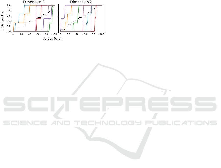
image on Figure 1); this gives an idea about what

does an ECD look like. Our methodology consists

in identifying the very similar and very close curves,

which would indicate that the two distributions are

very close in the feature space, and thus the clus-

ters alike. On the contrary, having no such proxim-

ity would indicate that the clusters are very different

(may be considered as a pledge of quality).

Figure 2: Example of ECDs, computed over BSOM’s clus-

ters (see rightmost image of Figure 1 for the clustering).

The dot black curve is the mean of all the colored ones.

3.3 Gathering of the Clusters

Once the clusters obtained and characterized, it is

time to process the results and see how to draw the

number of clusters from them.

As mentioned earlier, comparing two clusterings

sensu stricto is very difﬁcult, for there is no true uni-

versal indicator; we propose to use the Empirical Cu-

mulative Distributions instead, so as to describe the

clusters, and therefore use these characteristics for our

comparison. That being said, a problem remains: how

to compare two ECDs? Indeed, they are sets of val-

ues, and, as such, what characteristic to use to state

on their closeness? One may think about comparing

their mean through a distance measure, but this is very

weak; since we told that the position and the angle of

the slope are great indicators, they may also be worth

being compared, but this is not really clear, nor really

easy though (should the slope position weight more

than its angle? Is 5° a small or large difference?).

Therefore, we preferred interpreting the results as

graphical curves, which they actually are. To take all

their characteristics into account in a simple and very

representative fashion, we decided to compare their

shapes themselves: to do so, we followed the feel-

ing of Dubuisson and Jain, who consider the Haus-

dorff distance as one of the most appropriate distance

functions for shape recognition (Dubuisson and Jain,

1994). The Hausdorff distance compares two graph-

ical shapes (such as curves), and gives a closeness

score, the lower the closer. This distance is therefore

very-well adapted to our purposes, and has the advan-

tage of being simple while also highly representative.

For two discretized shapes P = {p

}

i∈[[1,N

]]

and

Q = {q

}

j∈[[1,N

]]

, the Hausdorff distance sets a point

in P and searches for the minimal distance between it

and any point in Q; it does so for any point in P and

takes the maximal value among all of these minimal

distances. Since the minimum and maximum are not

symmetric, this operation must be done the other way

round by exchanging P and Q. Finally, so as to obtain

a symmetric distance, the Hausdorff distance takes the

maximum between both. It is given by formula (5).



P,Q



= max



h(P,Q),h(Q,P)



(5)

where h(X,Y ) is the maximal value of the minimal

distances between sets X and Y, as given by 6. Notice

that generally h(X,Y ) ̸= h(Y, X ) (no symmetry).

h(X,Y ) = max

x∈X



min

y∈Y



d(x, y)





(6)

This deﬁnition has the drawback of ignoring most

values (only the maximum is considered); to compen-

sate that, (Dubuisson and Jain, 1994) proposed the

Modiﬁed Hausdorff Distance (MHD), which replaces

the maximum by a mean in the deﬁnition of h, more

representative of the shapes, as given by (7).

MHD

(X,Y ) =

|X|

∑

x∈X

min

y∈Y



d(x, y)



(7)

The ﬁnal deﬁnition of the MHD remains (5), but

using h

MHD

instead of h.

The (Modiﬁed) Hausdorff Distance is just an indi-

cator on the resemblance of two shapes: it is pairwise.

In our case, we have K clusters, therefore this distance

must be computed for any pair of cluster’s empirical

cumulative distributions, and that in any of the space’s

dimension. As a consequence, all these distances can

be gathered in a square matrix M ∈ R

K×K

; since the

MHD is built to be symmetric, the matrix will be sym-

metric as well, and since the MHD between a shape

and itself is null



(X, X) = 0



, its diagonal will be

full of zeroes, as shown by (8).

M =







ECD

··· ECD

ECD

0 d

(1,2)

··· d

(1,K)

ECD

(2,1)

0 ··· d

(2,K)

ECD

(K,1)

(K,2)

··· 0







(8)

where d

(i, j)

is the (Modiﬁed) Hausdorff Distance be-

tween ECD

and ECD

: d

(i, j)

= d



ECD

,ECD



Finally, once this matrix fulﬁlled, we propose to

use it to estimate the empirically optimal number of

clusters of the database. Indeed, if a value is low, it

means that the curves are graphically close, and thus

the data distributions are physically close alike, and

ETCIIM 2022 - International Workshop on Emerging Trends and Case-Studies in Industry 4.0 and Intelligent Manufacturing

284

therefore the clusters very likely belong to the same

database’s sub-region: merging them would probably

increase the clustering’s representativeness.

From there raises the question of how to con-

nect the ECDs with each other; indeed, there is often

many possible conﬁgurations. Consider the scenario

of three clusters aligned, regularly spaced of a Haus-

dorff distance α, as shown below:

α α

The corresponding matrix of the ECDs would

therefore be the following:

M =





0 α 2α

α 0 α

2α α 0





Assuming α is low, pairs {C

} and {C

}

are two possible candidates for merging. Nonethe-

less, the question to know what to do with C

remains:

since it belongs to two different pairs, should it be

merged with C

or with C

? From there, four possi-

bilities appear: 1- Do nothing; 2- Fuse C

with C

;

3- Fuse C

with C

; 4- Fuse the three clusters as one

(but is 2α a low enough distance?). This simple ex-

ample shows the problematic we are facing: there are

different cases, and there is no universal solution to it

(incidentally, this is the main problem with hierarchi-

cal clustering). To handle that, we propose to adopt a

Region Growing approach (Rabbani et al., 2006).

Indeed, this hierarchical clustering method draws

a point, assimilates it to a cluster’s barycenter, then

aggregates all the surrounding points at a maximum

distance of ρ, repeats this procedure for each one of

these neighbors, and continues to do so until there is

no more point at a maximum distance of ρ from any

point of this cluster not belonging to it or to any other

cluster. Once this cluster built, the procedure is re-

peated anew with another not-yet-assigned point, un-

til all the database’s points are categorized. This pro-

cedure can be serial (concurrent), by starting a new

cluster only when the last one has been completely

built, or it can be parallel, by building several clus-

ters at the same time. The ﬁrst ensures large clusters,

whilst the second leads to more, smaller of them.

Region growing can be considered in two ways:

either the data are truly fused into real entities (clus-

ters), or they can just be linked to one another, some-

how forming a map. Even though the two methods are

all the same, the second is more graphical, and thus

can ease the reading; in our case, the idea is to create

a graph whose nodes are the ECDs (or equivalently

the clusters), and the edges represent the connections

between them when they are less distant than ρ.

We propose to use this procedure to gather the

ECDs, which has the advantage of being efﬁcient and

proposing a solution to the above problem. In our

case, assuming α is low (i.e., α ≤ ρ), C

will be linked

to C

on the one hand, and C

will be linked to C

the other hand. As a consequence, we will get the or-

ganized set {C

}, meaning that C

will be in-

directly linked to C

through the intermediary of C

Following this procedure, Figure 3 gives an ex-

ample of conﬁgurations we could have (assuming the

arrows represent distances lower that ρ).

Group 1

Group 2

Group 3

Group 4

Figure 3: Example of region growing clustering and the re-

sulting cluster’s ECDs mapping.

Region growing clustering aims to identify the

sub-regions of the feature space, which is actually the

basis of the estimation of the number of clusters. In-

deed, blindly attempting to ﬁnd the correct clusters,

with no knowledge provided upstream, is like trying

to ﬁnd a needle in a haystack: nonetheless, it is much

easier to just search for the sub-regions of the space

instead of the true clusters. In reality, most clustering

methods work this way: they are based on the notion

of attraction, represented by the barycenters; that is

called their Region Of Inﬂuence (ROI), i.e., the area

around them within which any point can be aggre-

gated to them. This last point justiﬁes our choice in

the gathering of the ECDs by region growing.

Finally, our estimation of the number of clusters is

the number of subgroups built from the ECDs, eventu-

ally gathered by following a region growing approach.

This can be done by just reading the matrix of the

ECDs M; indeed, if a value is low (according to a

threshold), it means that the two corresponding ECDs

(and thus clusters) can be connected to one another.

As such, to operate the region growing clustering, one

just has to create a map of all the clusters and link

them within; to do so, just ﬁnd the lowest values of

the matrix and add the corresponding connections to

ECD Test: An Empirical Way based on the Cumulative Distributions to Evaluate the Number of Clusters for Unsupervised Clustering

285

the map. Once done, the map can be easily read, and

the estimated optimal number of clusters is simply the

number of disconnected groups (regions).

3.4 Summary of the Proposal

To make clearer our methodology, this subsection

aims to summarize the previous ones. Its different

steps can be enumerated as follows:

1. Cluster a database using an unsupervised, data-

driven clustering method from the state-of-the-art,

with a high value set for the number of clusters. It

may be the K-Means, the Self-Organizing Maps

or the Bi-Level SOMs for instance.

2. Compute the ECDs for every cluster, in every di-

mension, using (4).

3. Compute the MHDs between any pair of ECDs

using (5) and (7), and gather all of them within a

matrix, such as shown in (8).

4. Gather all the MHDs of the matrix into compact

and similar regions using Region Growing clus-

tering, as shown in Figure 3.

5. Read the so-built cluster’s ECDs mapping: the es-

timated number of clusters K

′

of the database is

the number of regions identiﬁed.

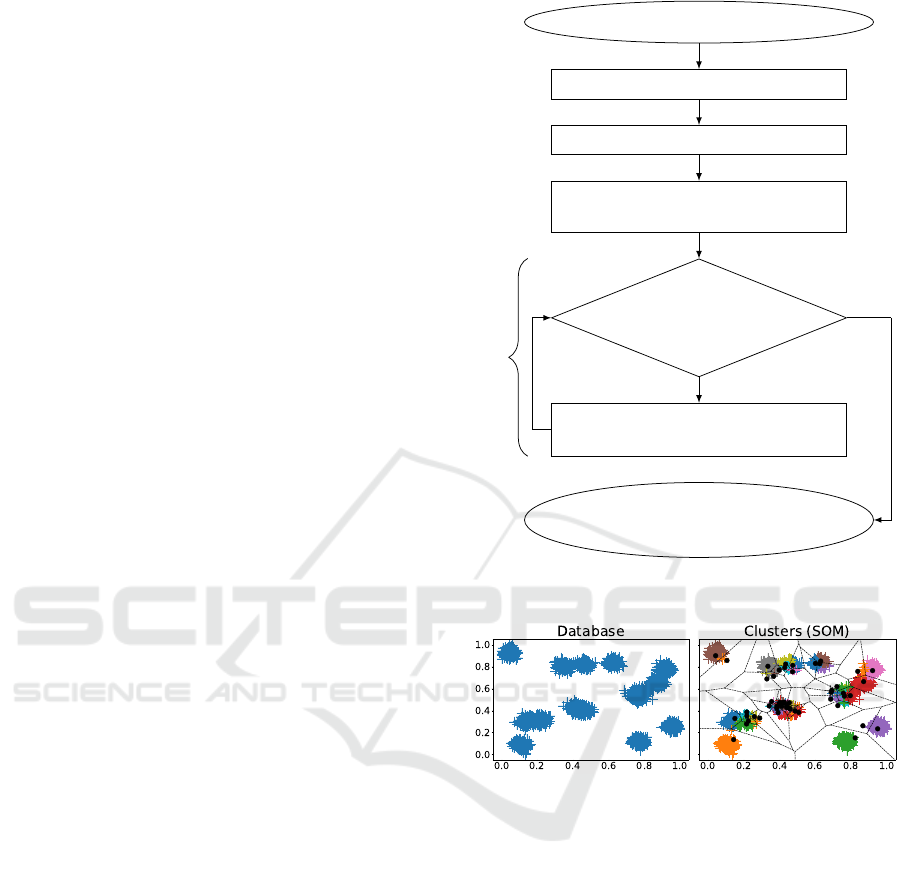
All this methodology is graphically summarized

in a ﬂowchart as of Figure 4.

4 RESULTS

In this section, we will apply the proposed method to

an academic dataset in order to show how it works

step by step and how to interpret each of them. We

will then apply this methodology to real industrial

data to show its potential in real conditions.

4.1 Academic Dataset

To illustrate our approach, consider ﬁrst a simple but

truly didactic example: a set of ﬁfteen 2D Gaussian

distributions. We will mainly use the Self-Organizing

Map, but we will also try the K-Means and BSOM.

Figure 5 depicts both the original database (left) and

the clustered data using a 10 × 10 SOM (right). We

remind that the ﬁrst step is to break the input database

in very small pieces, whence the large number of

SOM’s grid’s nodes (100). Notice that the objective

number of clusters should be a dozen, depending on

the accuracy one wants to achieve; indeed, for in-

stance, on the right of the leftmost image on the ﬁgure

(the dataset), three clusters are clearly overlapping,

Database to analyse

Cluster the database (K high)

Compute the ECDs for each cluster

Build the matrix of the MHDs &

Initialize the linkage map (no edge)

∃(i, j), d

(i, j)

≤ ρ

& (i, j) /∈ map

Add edge between

ECD

and ECD

in map

Estimate K

′

as the num-

ber of groups in map

Yes

Region Growing

Figure 4: Flowchart of the proposed method for empirical

estimation of the number of clusters in a database.

Figure 5: Results of the SOMs with a 10 × 10 grid.

thus should they be considered as different or as one

unique data group? Depending on the accuracy, one

may identify up to 9-12 different groups; this range of

numbers is the objective of our proposed method.

The SOM led to 48 empty clusters (this is made

possible by the learning procedure), which will not

be considered in the following. As such, Figure 6 de-

picts the Empirical Cumulative Distributions of the

52 nonempty clusters. There are too many curves

to clearly identify the different groups; nonetheless,

this image is interesting for it shows what do ECDs

look like with real data, and to remember that they

must be computed in any dimension, whence the two

subgraphs. Moreover, in our approach, an important

thing to remind is that to consider two ECDs as close,

they must be in all dimensions. For instance, the pink

and violet curves at the extreme right in the leftmost

image are very close in that dimension, but not in the

ETCIIM 2022 - International Workshop on Emerging Trends and Case-Studies in Industry 4.0 and Intelligent Manufacturing

286

Figure 6: ECDs of the clustering (rightmost image of Fig-

ure 5). The dot black curve is the mean of all the colored

curves, each corresponding to the ECDs of a unique cluster.

second one: therefore, they can not be considered as

close, whence the validation of the closeness in every

dimension, and the ﬁnal comparison of the matrices

of the MHDs in all dimensions.

Now that the clusters have been built and that their

ECDs have been computed, their Modiﬁed Hausdorff

Distances must be computed and gathered within the

MHD Matrices, for each dimension. Table 1 presents

a part of these matrices: M

and M

are these ma-

trices compared term by term to a threshold ρ, fol-

lowing region growing clustering; if a pair of ECDs

has a MHD lower than ρ, this pair is tagged with the

Boolean True (noted T in the rightmost matrices), and

False else (noted F). Finally, to test if two ECDs are

actually close, the ﬁnal matrix of the pairs is given by

logical and &: M = M

& M

, as depicted on Table 2.

This matrix allows to gather the pairs into full

groups of ECDs, by region growing clustering: two

pairs are connected if they share at least one com-

mon ECD. For instance, {11,19} and {11,22} are

two such pairs, since they share ECD

. Finally,

the formed groups are the following: {10,18} in

red, {11,19,22} in green, {14,15, 20} in orange, and

{12,16,21,23,24} in blue. These pairs are mapped

as of Figure 7; notice that connections are completed

with dot edges with the whole matrix (for instance,

ECD

and ECD

are not connected in Table 2, but

they actually are in the full matrix). In short words,

that means that for 14 clusters considered here, they

actually form 5 groups: the number of clusters here

should therefore be 5 (the blue, red, green and orange

ones, plus the isolated cluster 13).

Finally, by reading the full matrix and creating the

full map, we obtain the following groups: {1}, {2},

{3}, {4, 44}, {5, 41}, {6, 31}, {14, 15, 20}, {0,

11, 19, 22, 28, 39, 51}, {7, 10, 18, 27, 29, 36, 45,

48}, {8, 9, 13, 32, 34, 40, 42, 47}, {12, 16, 17, 21,

23, 24, 25, 26, 30, 33, 35, 37, 38, 43, 46, 49, 50}.

These groups are the ﬁnal ones, i.e., the compact re-

gions of the space; by enumerating these regions (thus

groups), we obtain our estimate for the number of

clusters, whence K

′

= 11, which is in our objective

range of 9-12, and especially very close to the real

number of non-overlapping clusters.

Finally, to generalize a little, Table 3 gathers

the mean estimated number of clusters using SOM,

BSOM and K-Means. Each method has been run 100

times, and some statistics are presented in the table.

The three methods provide similar estimates, liv-

ing in the same range. It is hard to state on which is

the best, for it depends on the user’s needs. Indeed, as

discussed with Figure 5, several numbers of clusters

can be accepted: 9-10 if one only thinks by full re-

gions (possible clusters’ overlapping), or 12-14 if one

wants more accurate groups. As such, depending on

the accuracy, one method can be preferred over the

two others. For instance, the K-Means gave the low-

est number of clusters, with a very low standard devi-

ation: it can be used to get consistent results; on the

contrary, BSOM gave about 12 clusters, which is ac-

tually the closest to the reality (cluster by cluster): it

can be used to get clearer clusters, with ﬁner borders.

Moreover, we have not talked about cluster’s quality,

but maybe these values are all great and are the most

appropriate for their respecting clustering method.

Anyway, these results seem very promising, and

indicate that the proposed method works very well, at

least with this academic example. Moreover, it proved

to be resilient to the clustering method used: there is

no huge gap with the results when using a method or

another, which is somehow reassuring.

4.2 Real Industrial Data

Now that the method has been validated over an aca-

demic dataset, so as to test it and also to show step

by step how it works, it is time to apply it to a real

context, i.e., real industrial data. These data were pro-

vided to us by Solvay

, a chemistry plant specialized

in Rare Earth specialties extraction. They are one of

the HyperCOG partners, a H2020 European project

whose main aim is to study the feasibility of the Cog-

nitive plant, i.e., the intelligent and autonomous in-

dustry of tomorrow (Industry 4.0).

15 20

Figure 7: Mapping of the MHDs.

ECD Test: An Empirical Way based on the Cumulative Distributions to Evaluate the Number of Clusters for Unsupervised Clustering

287

Table 2: Final matrix of the closeness of the ECDs, for all

dimensions, given as the logical and between all the cor-

responding matrices in any dimension. The True T have

been regrouped by color, following region growing cluster-

ing: one color per ﬁnal group (region).

& M







18 19 20 21 22 23 24

10 T F F F F F F

11 F T F F T F F

12 F F F T F T T

13 F F F F F F F

14 F F T F F F F

15 F F T F F F F

16 F F F T F F T







The process we are studying at Solvay

is the

Rare Earth separation from raw material; this step is

performed in what is called a ”battery”. The data we

will work with in this section came from one of these

batteries: they were recorded over seven work weeks,

at a rate of one per minute, for a total of 65,505 data

samples, over 14 sensors (and thus as many dimen-

sions in the feature space). For conﬁdentiality con-

cerns, these data have been normalized. Following

our work (Molini

e et al., 2022), there should be about

7-10 real behaviors in this battery, and thus as many

objective clusters (one per real system’s behavior).

Table 3: Estimated number of clusters using different clus-

tering methods after 100 runs each, with 100-node grids for

SOM and BSOM, and K = 50 for the K-Means.

Method Mean Std Min Max

K-Means 10.04 0.86 9 12

SOM 10.21 1.44 8 14

BSOM 12.21 1.18 10 16

This range of values is therefore our objective here.

Figure 8 depicts two of these sensors over time

(left), their respective feature space on the top right

hand corner (sensor 2’s data against sensor 1’s), and

the corresponding clustering below, using the BSOM.

Notice that the clustering was performed using all the

sensors/dimensions, but only two are depicted for the

sake of conciseness.

BSOM used 10 SOMs, with 100 nodes each; the

ﬁnal clustering contains 61 nonempty clusters, with

which we will deal. The ECDs have been computed

for every cluster, and then compared to one another

using the MHD, and the ﬁnal state matrix of all the

pairs’ MHDs has been built. Table 4 gives a por-

tion of that matrix, where, anew, T corresponds to

a close pair, and F to a distant one. The sensors’

tag numbers have been added on the top and left as

small italic numbers. The colors corresponds to the

Table 1: Part of the MHDs matrices for every dimension (left) and the state on the closeness for every pair of ECDs (right), in

which T means that the two ECDs involved in the corresponding pair are close, and F else. The indexes of the cluster’s ECDs

are indicated at the very start of every row, and at the top of every column as small italic numbers.

Dimension 1 M

z }| {







18 19 20 21 22 23 24

10 0.90 9.20 2.50 0.30 10.2 1.20 1.60

11 7.00 0.40 17.0 9.10 0.50 5.60 4.50

12 0.50 7.90 3.10 0.50 8.90 0.60 1.00

13 16.3 37.9 5.60 12.7 39.8 17.7 19.3

14 6.20 21.0 0.80 4.00 22.4 6.90 7.90

15 6.20 21.1 0.70 4.00 22.6 7.00 8.00

16 0.50 5.40 4.50 1.10 6.30 0.40 0.50







≤ ρ =







18 19 20 21 22 23 24

10 T F F T F T T

11 F T F F T F F

12 T F F T F T T

13 F F F F F F F

14 F F T F F F F

15 F F T F F F F

16 T F F T F T T







Dimension 2 M

z }| {







18 19 20 21 22 23 24

10 0.40 26.9 0.30 22.9 33.8 23.1 19.5

11 32.3 0.60 31.1 1.90 0.60 1.30 2.10

12 23.0 1.00 22.1 0.50 2.60 0.40 0.50

13 12.3 6.30 11.6 4.50 9.80 4.60 3.10

14 0.60 25.8 0.50 21.9 32.7 22.2 18.5

15 0.50 30.3 0.60 26.1 37.7 26.4 22.4

16 19.6 1.70 18.7 0.80 3.70 3.50 0.30







≤ ρ =







18 19 20 21 22 23 24

10 T F T F F F F

11 F T F F T T F

12 F T F T F T T

13 F F F F F F F

14 T F T F F F F

15 T F T F F F F

16 F F F T F F T







ETCIIM 2022 - International Workshop on Emerging Trends and Case-Studies in Industry 4.0 and Intelligent Manufacturing

288

Figure 8: Possible clustering obtained with real industrial

data. On the left, the two sensor’s data over time; on the

right, their corresponding feature space (sensor 2’s data

against sensor 1’s) and the clustering given by BSOM.

Table 4: Example of the all-dimension state matrix.

M =







44 45 46 47 48 49 50

33 F F F F F T T

34 F F F F F F T

35 F T F F F F F

36 F F F F F F T

37 F F F F F F F

38 F T F F F F F

39 T F F T F F F







groups formed by region growing: {33,34,36,49,50}

in blue, {35,38,45} in green, and {39, 44, 47} in red.

The corresponding map is depicted on Figure 9,

where the numbers correspond to the ECDs (e.g.,

”34” means ECD

); the plain edges are that drawn

from the matrix, and the dotted edges are that drawn

when considering all the 61 clusters.

The results mean that there actually are 5 groups:

the colored ones, plus the isolated {37} and {48}.

Finally, the full groups are the following (”x-y” means

all values between x and y): {37}, {43}, {53}, {27,

42, 48}, {28, 35, 38, 45, 60}, {2-5, 16, 18, 19, 23,

30, 32, 41, 46, 54, 58}, {0, 1, 6-15, 17, 20-22, 24-26,

29, 31, 33, 34, 36, 39, 40, 44, 47, 49-52, 55-57, 59}.

As a consequence, there are 7 groups of clusters, and

therefore, the estimated number of clusters is K

′

= 7,

which is actually the one we were expecting.

33 36

Figure 9: Example of mapping of the Battery.

Table 5: Number of regions obtained with the Solvay’s data,

using each of the three clustering methods, run 100 times,

with 100 nodes for SOM and BSOM, and 50 for K-Means.

Method Mean Std Min Max

K-Means 3.9 0.98 2 6

SOM 7.98 2.05 3 12

BSOM 8.46 2.54 4 15

Eventually, Table 5 compares the results obtained

when using the three clustering methods introduced

earlier, run 100 times: the mean, standard deviation,

minimum and maximum for each method.

The results of this table are close to that drawn

from the academic dataset: BSOM is the closest to re-

ality, with the best range, but a high scattering, closely

followed by SOM; the K-Means has the least scat-

tered results, but the number of regions identiﬁed is a

little low. That being said, all the three methods have

provided acceptable estimates (no aberration nor out-

liers), which conﬁrms the universality of our method.

5 CONCLUSION

Unsupervised clustering is a blind approach which

aims to point out the similarities and hidden patterns

of an unknown database. They are automatic, but gen-

erally require an important parameter as of the ex-

pected number of clusters. This parameter must be

set manually, and the choice of one value over an-

other may change the clustering’s representativeness

in depth. In this paper, we have addressed the prob-

lem of the automatic estimation of the empirical op-

timal number of clusters to be set as meta-parameter

for an unsupervised, data-driven clustering method.

To that purpose, we propose the ECD Test, which

aims to estimate the empirically most suited number

of clusters. Whilst most approaches from literature

operate several clusterings by varying the number of

clusters, and by selecting that achieving the best re-

sults, we rejected that idea, for it is closer to a true

brute-force clustering rather than a real estimation

of the number of clusters. Our method relies on a

hierarchical aggregation of the characteristics of the

database so as to propose a judicious estimate.

Indeed, we propose to operate a unique clustering,

with a high number of clusters, compute the Empirical

Cumulative Distributions to characterize the clusters,

and ﬁnally bring the clusters together according to the

closeness of their respective ECDs. To do so, we com-

pute the Modiﬁed Hausdorff Distance between any

couple of two ECDs, and gather all these measures

into a unique matrix, whose values are compared to a

threshold: if a value is low, then the involved ECDs

ECD Test: An Empirical Way based on the Cumulative Distributions to Evaluate the Number of Clusters for Unsupervised Clustering

289

(and then clusters) are considered as close. Finally, all

these measures are linked to one another into a map

by region growing clustering, allowing to rebuild the

regions of the feature space. The number of isolated

groups of clusters is somehow the number of regions

of the feature space, and therefore a very good esti-

mate for the optimal number of clusters.

We assessed this methodology over an academic

dataset consisting in ﬁfteen 2D-Gaussian Distribu-

tions, and then over real industrial data. In both cases,

we found back about the number of clusters we had

expected, i.e., a ten in both cases. We tested three

clustering methods (K-Means, SOMs and Bi-Level

SOMs) to show the resilience of our methodology,

which proved to be highly reliable in any context,

even with unsupervised data-driven approaches.

The ECD Test tool is very helpful to prepare the

ground for some sort of next steps. In our next works,

we will endeavor to use it in wider situations, and to

use it so as to get the best clustering as possible on

real datasets. A great and accurate clustering is of

major importance in many contexts, such as multi-

modeling the system under consideration (one local

model for each cluster): this is the solution we are ac-

tually working on, and the reason why we addressed

the problem raised in this paper.

ACKNOWLEDGEMENTS

This paper received funding from the European Union

Horizon 2020 research and innovation program under

grant agreement N°695965 (project HyperCOG).

REFERENCES

Amorim, R. and Hennig, C. (2015). Recovering the number

of clusters in data sets with noise features using fea-

ture rescaling factors. Information Sciences, 324:126–

145.

Defays, D. (1977). An efﬁcient algorithm for a complete

link method. Comput. J., 20:364–366.

Dhillon, I., Guan, Y., and Kulis, B. (2004). Kernel k-means,

spectral clustering and normalized cuts. KDD-2004 -

Proceedings of the Tenth ACM SIGKDD International

Conference on Knowledge Discovery and Data Min-

ing, 551-556.

Dubuisson, M. and Jain, A. (1994). A modiﬁed hausdorff

distance for object matching. In Proceedings of 12th

International Conference on Pattern Recognition, vol-

ume 2, pages 566,567,568, Los Alamitos, CA, USA.

IEEE Computer Society.

Goutte, C., Hansen, L., Liptrot, M., and Rostrup, E. (2001).

Feature-space clustering for fmri meta-analysis. Hu-

man brain mapping, 13:165–83.

Hassani, H. and Silva, E. S. (2015). A kolmogorov-smirnov

based test for comparing the predictive accuracy of

two sets of forecasts. Econometrics, 3(3):590–609.

Honarkhah, M. and Caers, J. (2010). Stochastic simula-

tion of patterns using distance-based pattern model-

ing. Mathematical Geosciences, 42:487–517.

Kohonen, T. (1982). Self-organized formation of topolog-

ically correct feature maps. Biological Cybernetics,

43(1):59–69.

Lloyd, S. P. (1982). Least squares quantization in pcm.

IEEE Trans. Inf. Theory, 28:129–136.

Marutho, D., Hendra Handaka, S., Wijaya, E., and Muljono

(2018). The determination of cluster number at k-

mean using elbow method and purity evaluation on

headline news. In 2018 International Seminar on Ap-

plication for Technology of Information and Commu-

nication, pages 533–538.

Molini

e, D. and Madani, K. (2021). Characterizing n-

dimension data clusters: A density-based metric for

compactness and homogeneity evaluation. In Pro-

ceedings of the 2nd International Conference on In-

novative Intelligent Industrial Production and Logis-

tics – IN4PL, volume 1, pages 13–24. INSTICC,

SciTePress.

Molini

e, D., Madani, K., and Amarger, V. (2022). Cluster-

ing at the disposal of industry 4.0: Automatic extrac-

tion of plant behaviors. Sensors, 22(8).

Molini

e, D. and Madani, K. (2022). Bsom: A two-

level clustering method based on the efﬁcient self-

organizing maps. In 6th International Conference on

Control, Automation and Diagnosis (ICCAD). [Ac-

cepted but not yet published by July 29, 2022].

Molini

e, D., Madani, K., and Amarger, C. (2021). Identi-

fying the behaviors of an industrial plant: Application

to industry 4.0. In Proceedings of the 11th Interna-

tional Conference on Intelligent Data Acquisition and

Advanced Computing Systems: Technology and Ap-

plications, volume 2, pages 802–807.

Pelleg, D. and Moore, A. (2002). X-means: Extending k-

means with efﬁcient estimation of the number of clus-

ters. Machine Learning.

Rabbani, T., Heuvel, F., and Vosselman, G. (2006). Seg-

mentation of point clouds using smoothness con-

straint. International Archives of Photogrammetry,

Remote Sensing and Spatial Information Sciences, 36.

Rousseeuw, P. (1987). Silhouettes: A graphical aid to the in-

terpretation and validation of cluster analysis. Journal

of Computational and Applied Mathematics, 20:53–

65.

Rybnik, M. (2004). Contribution to the modelling and the

exploitation of hybrid multiple neural networks sys-

tems : application to intelligent processing of infor-

mation. PhD thesis, University Paris-Est XII, France.

Sibson, R. (1973). Slink: An optimally efﬁcient algorithm

for the single-link cluster method. Comput. J., 16:30–

34.

Simard, R. and L’Ecuyer, P. (2011). Computing the two-

sided kolmogorov-smirnov distribution. Journal of

Statistical Software, 39(11):1–18.

Tibshirani, R., Walther, G., and Hastie, T. (2001). Estimat-

ing the number of clusters in a data set via the gap

statistic. Journal of the Royal Statistical Society Se-

ries B, 63:411–423.

ETCIIM 2022 - International Workshop on Emerging Trends and Case-Studies in Industry 4.0 and Intelligent Manufacturing

290