An Effective Two-stage Noise Training Methodology for Classification of
Breast Ultrasound Images
Yiming Bian
a
and Arun K. Somani
b
Department of Electrical and Computer Engineering, Iowa State University, Ames, Iowa, U.S.A.
Keywords:
Noise Training, Single-noise Training, Mix-noise Training, Breast Ultrasound Image, Image Classification.
Abstract:
Breast cancer is one of the most common and deadly diseases. An early diagnosis is critical and in-time treat-
ment can help prevent the further spread of cancer. Breast ultrasound images are widely used for diagnosis,
but the diagnosis heavily depends on the radiologist’s expertise and experience. Therefore, computer-aided di-
agnosis (CAD) systems are developed to provide an effective, objective, and reliable understanding of medical
images for radiologists and diagnosticians. With the help of modern convolutional neural networks (CNNs),
the accuracy and efficiency of CAD systems are greatly improved. CNN-based methods rely on training with
a large amount of high-quality data to extract the key features and achieve a good performance. However, such
noise-free medical data in high volume are not easily accessible. To address the data limitation, we propose
a novel two-stage noise training methodology that effectively improves the performance of breast ultrasound
image classification with speckle noise. The proposed mix-noise-trained model in Stage II trains on a mix of
noisy images at multiple different intensity levels. Our experiments demonstrate that all tested CNN models
obtain resilience to speckle noise and achieve excellent performance gain if the mix proportion is selected
appropriately. We believe this study will benefit more people with a faster and more reliable diagnosis.
1 INTRODUCTION
Breast cancer is one of the most deadly diseases for
people, especially women, all around the world. Cur-
rently, ultrasound scanning is widely adopted as a
complimentary diagnose method. However, the di-
agnosis heavily depends on the experience of the ra-
diologist, which may be slow, expensive, and some-
times not as accurate for everyone. For better ultra-
sound image understanding, CAD systems are devel-
oped using machine learning algorithms. It also helps
to overcome the shortcomings of ultrasound diagno-
sis and helps doctors improve the accuracy and effi-
ciency of diagnosis (Wang et al., 2021). The use of
ultrasound-based CAD for the classification of tumor
diseases provided an effective decision-making sup-
port and a second tool option for radiologists or diag-
nosticians (Liu et al., 2019).
CNN-based studies have pushed great progresses
in medical image classification field. Most backbone
CNN architectures were proposed with the develop-
ment of ImageNet Large Scale Visual Recognition
a
https://orcid.org/0000-0002-8725-3603
b
https://orcid.org/0000-0002-6248-4376
Challenge (ILSVRC) (Russakovsky et al., 2015). In
2009, a large database, which contains over 14 mil-
lion hand-annotated images, designed for visual ob-
ject recognition research called ImageNet was pre-
sented by Li Fei-Fei et al. (Deng et al., 2009). In
the follwoing year, ImageNet project began an an-
nual contest called ILSVRC. This challenge uses a
subset of ImageNet that has 1, 000 non-overlapping
classes of objects. As it is commonly acknowledged
that the average recognition capability of human has
a top-5 error rate of 5%, the winner in 2015, ResNet
(He et al., 2016), beat human-level object recogni-
tion capability for the first time with a top-5 error
rate of 3.6%. The state-of-the-art model, Florence
(Yuan et al., 2021), achieved an extraordinary top-5
error rate of 0.98%. As the annual champion models
having a deeper and deeper architecture, deep neural
networks have proved to be practical and effective in
image classification tasks. All of these intriguing fig-
ures and achievements indicate that the improvement
of classification accuracy on high-quality images is
not a big challenge anymore.
However, image classification in medical areas
still faces great difficulties. The shortage of large
volume of high-quality medical data is an undeniable
Bian, Y. and Somani, A.
An Effective Two-stage Noise Training Methodology for Classification of Breast Ultrasound Images.
DOI: 10.5220/0011553000003335
In Proceedings of the 14th International Joint Conference on Knowledge Discovery, Knowledge Engineering and Knowledge Management (IC3K 2022) - Volume 1: KDIR, pages 83-94
ISBN: 978-989-758-614-9; ISSN: 2184-3228
Copyright
c
 2022 by SCITEPRESS – Science and Technology Publications, Lda. All rights reserved
83

predicament. Ultrasound medical datasets are more
difficult to obtain as the annotation of medical images
requires significant professional medical knowledge
(Liu et al., 2019). Moreover, most patients prefer
to keep their health data private, which makes public
medical data a very rare resource. Another obstacle is
the medical data acquisition device difference. Not all
devices produce high-quality images that reflect key
features of the target object. Also, the complexity na-
ture of disease itself, such as massive amount of con-
tour patterns of a malignant tumor, prevents the med-
ical image annotation from totally reliable and poses
great challenges for a CNN model to generalize.
Given the fact that most medical data, including
ultrasound images, inevitably contain speckle noise
during the acquisition process. Noisy data is another
significant obstacle for CNN-based studies. After
years of studies, researchers have developed effective
despeckling techniques that improve the performance
of CNN models.
1.1 Related Work
Previous researchers have accomplished great out-
comes on speckle noise suppression while keeping the
edge information and preserving a high-quality con-
tour in breast ultrasound images. In (Bhateja et al.,
2014), Bhateja, Vikrant, et al. present a modified
speckle suppression algorithm using directional av-
erage filters for breast ultrasound images in homo-
geneity domain. Their simulation results show sig-
nificant performance improvement regarding speckle
noise removal and edge preservation. In (Virmani
et al., 2019), Virmani, Jitendra, and Ravinder Agar-
wal propose a detail preserving anisotropic diffusion
(DPAD) despecking filtering algorithm that optimally
reduces the speckle noise from ultrasound images by
retaining texture information and enhancing the tu-
mor edges. In (Chang et al., 2019), Chang, Yi, et
al. remove the noise in medical images from image
decomposition perspective. They treat the noise and
image components equally and propose a two-stage
CNN that models both the image and noise simul-
taneously. In (Li et al., 2022), Li, Xiaofeng, et al.
propose a fast speckle noise suppression algorithm in
breast ultrasound image using three-dimensional deep
learning. Their experiment results demonstrate that
the speckle noise suppression time is low, the edge
information is well preserved and the image details
are visible.
CNN-based methods were adopted for medical
image understanding. In (Liu et al., 2019), Liu,
Shengfeng, et al. review popular deep learning ar-
chitectures and thoroughly discuss their applications
in ultrasound image analysis such as classification,
detection and segmentation. In (Sarvamangala and
Kulkarni, 2021), Sarvamangala, D. R., and Raghaven-
dra V. Kulkarni provide a comprehensive survey
of applications of CNNs in medical image under-
standing such as X-ray, magnetic resonance imaging
(MRI), computed tomography (CT) and ultrasound
scanning. In (Daoud et al., 2019), Daoud, Moham-
mad I., Samir Abdel-Rahman, and Rami Alazrai in-
vestigate the use of deep features extraction and trans-
fer learning to enable the use of a pretrained CNN
model to achieve accurate classification of breast ul-
trasound images. Their results suggest that an ac-
curate breast ultrasound image classification can be
achieved with features extracted from the pretrained
CNN model and effective feature selection algo-
rithms.
Medical data scarcity problem is one of the great-
est obstacles in CNN-related researches. To mitigate
this issue, transfer learning has been adopted in ma-
jority of related studies. In (Kim et al., 2022), Kim,
Hee E., et al. provide actionable insights on how
to select backbone CNN models and tune them with
consideration of medical data characteristics. For ex-
ample, they suggest that the model should be fine-
tuned by incrementally unfreezing convolutional lay-
ers from top to bottom layers with a low learning rate.
In (Ayana et al., 2022), Ayana, Gelan, et al. propose
a multistage transfer learning algorithm and their re-
sults show the significant improvement in the classi-
fication performance of breast ultrasound images. In
(Wang et al., 2021), Wang, Yu, et al. review the data
preprocessing methods of medical ultrasound images,
including data augmentation, denoising and enhance-
ment. They explicitly mentioned that traditional ma-
chine learning methods are vulnerable to possible low
imaging quality and deep learning can reduce this im-
pact by extracting high-level features.
1.2 Contributions
In this work, we focus on improving the performance
of CNN models on classifying breast ultrasound im-
ages with speckle noise. We explore the impact of
noisy data training on noisy data classification. Fac-
ing the data shortage problem during our experiments,
we mitigate this issue and overcome class imbalance
problem by applying augmentation and oversampling
techniques. Finally, we propose a systematic two-
stage noise training methodology that improves the
classification performance of the selected CNN archi-
tectures on noisy data. Tested models show excellent
resilience to speckle noise after applying our method-
ology. We also provide empirical parameter choices
KDIR 2022 - 14th International Conference on Knowledge Discovery and Information Retrieval
84

for generating ultrasound images with artificial noise,
constructing noisy datasets, training networks and ob-
tain the model with the best performance.
The rest of the paper is organized as follows. Sec-
tion II provides preliminary knowledge of speckle
noise, deep convolutional networks and image classi-
fication. Our two-stage noise training methodology is
introduced in Section III. Section IV describes how all
the datasets are prepared and how the corresponding
CNN models are developed. We present our experi-
ments, results and detailed analysis in Section V. Con-
clusions and future research directions are discussed
in Section VI.
2 BACKGROUND
In this section, we provide prerequisite knowledge of
speckle noise, deep neural networks and image classi-
fication. Specifically, we answer the following ques-
tions: 1) how speckle noise is formed; 2) why speckle
noise is common in medical images; 3) how speckle
noise is simulated; 4) why deep neural networks are
effective on noise medical image processing; and 5)
what popular neural network architectures are in med-
ical image classification field.
2.1 Speckle Noise
Speckle is a common phenomenon in images ob-
tained by coherent imaging systems such as synthetic-
aperture radar (SAR) and ultrasound machines be-
cause the object surface is rough on the scale of
wavelength. The reflectivity function of the image
acquisition device produces scatterers. These scat-
tered signals add coherently, which forms the patterns
of constructive and destructive interference shown as
bright and dark dots in the image (Forouzanfar and
Abrishami-Moghaddam, 2011). In medical images,
especially ultrasound images, speckle noise is almost
inevitable because mainstream ultrasound machines
are coherent imaging systems, and human tissue and
lesion tissue have a rough surface. Fig. 1 shows an
SAR image of San Francisco, California and a breast
ultrasound image of a benign tumor. Speckle noise in
both images can be easily observed.
In our experiments, we simulate speckle noise us-
ing “imnoise()” function in MATLAB. This function
adds various synthetic noise to the input image. The
full documentation is available online by MathWorks
1
https://www.jpl.nasa.gov/images/pia01751-space-
radar-image-of-san-francisco-california
2
https://www.kaggle.com/datasets/aryashah2k/breast-
ultrasound-images-dataset
(a) (b)
Figure 1: (a) A Space Radar Image of San Francisco, Cali-
fornia (Cropped): It was acquired by the Spaceborne Imag-
ing Radar-C and X-Band Synthetic Aperture Radar (SIR-
C/X-SAR) aboard space shuttle Endeavour on orbit 56 on
October 3, 1994. It is available online by NASA/JPL-
Caltech
1
. (b) A Breast Ultrasound Image of a Benign
Tumor (Cropped): This image is included in a public
dataset called Breast Ultrasound Image Dataset (BUSI)
(Al-Dhabyani et al., 2020). It is stored under the folder
‘BUS/benign’ with a filename of ‘000087’. The whole
dataset is available online by Kaggle
2
.
Help Center
3
. Speckle noise is multiplicative and it
is generated using Equation 1, where the input image
(I
img
) is a matrix of integer numbers, each ranging
from 0 to 255. Gray-scale images and RGB images
have a third dimension of 1 and 3 respectively. The
multiplication is element-wise and the synthetic noise
(η) is uniformly distributed with mean (µ) equals to
0 and variance (σ
2
) to be specified. The variance,
σ
2
, controls the intensity of noise. The output im-
age (O
img
) shares the same dimension with the input
image (I
img
).
O
img
= I
img
+ ηI
img
(1)
The value of an output pixel (o
pixel
) is determined
by σ
2
and the input pixel value (i
pixel
). Their quantita-
tive relationship is given in Equation 2. The range of
o
pixel
is from 0 to 255. When o
pixel
is out of the range,
it is automatically bounded to the nearest marginal
value, thus either 0 or 255.
o
pixel
= i
pixel
+
√
12σ
2
×i
pixel
×[rand(0, 1)−0.5] (2)
As the synthetic noise (η) is uniformly dis-
tributed, thus η ∼ U(a, b), where a and b are the
minimum and maximum values of η. The mean
(µ) and variance (σ
2
) can be expressed using a
and b as given in Equation 3. Then we have
√
12σ
2
= 2b −2µ. Since µ = 0, it is simplified to
√
12σ
2
= 2b. The range [a, b] can be expressed as
2bm, where m is a random value and m ∈ [−0.5, 0.5].
The expression 2bm can be written as
√
12σ
2
×
[rand(0, 1) −0.5], which explains the multiplication
part of Equation 2.
3
https://www.mathworks.com/help/images/ref/imnoise
An Effective Two-stage Noise Training Methodology for Classification of Breast Ultrasound Images
85

(
µ =
1
2
(a + b)
σ
2
=
1
12
(b −a)
2
(3)
Depending on the source of ultrasound images,
some are stored as gray-scale while other are RGB
images, although they all appear to be gray-scaled. It
causes issues in both adding artificial noise and pro-
cessing using CNN models. Adding speckle noise
to an RGB ultrasound image generates noise pixels
with colors, which degrades the simulation quality.
Therefore, it is necessary to convert the RGB image
to gray-scale. On the other hand, the vast majority of
CNN models take an RGB image as input. We ad-
dress both problems by first converting RGB images
to gray-scale and add artificial speckle noise. Then
we duplicate two more channels and form them into
the proper size that is compatible to a CNN’s input.
2.2 Deep Neural Networks and Image
Classification
A concise introduction to deep neural network has
been provided in (Dodge and Karam, 2016). The
big picture of deep learning, convolutional neural net-
work, image understanding with deep convolutional
networks were discussed in (LeCun et al., 2015). A
large amount of research has been done on applying
deep neural network to image classification tasks such
as aforementioned models in ILSVRC. All of them
were trained on a subset of ImageNet, which contains
1, 000 non-overlapping classes and has over 1.2 mil-
lion sample images.
In medical area, however, the lack of large vol-
ume of high-quality data poses great challenges.
As introduced above, images with noise are com-
mon in medical area during the acquisition process.
Apart from noise suppression techniques, machine-
learning-based methods are gaining more popularity
in recent years. Traditional neural networks are vul-
nerable to low quality images. To address this issue,
neural networks with deeper levels are developed as
they can extract high-level features and improve the
classification performance.
In medical image processing area, some popular
backbone CNNs are well-experimented and explored.
For example, AlexNet is the main focus in (Nawaz
et al., 2018) (Masud et al., 2021). ResNet is stud-
ied in (Jiang et al., 2019) (Al-Haija and Adebanjo,
2020) (Virmani et al., 2020) (Yap et al., 2020) (Yu
et al., 2020) and VGG16 provides the best perfor-
mance in (Moon et al., 2020) (Hadad et al., 2017) (Ja-
hangeer and Rajkumar, 2021) (Albashish et al., 2021)
(Jahangeer and Rajkumar, 2021).
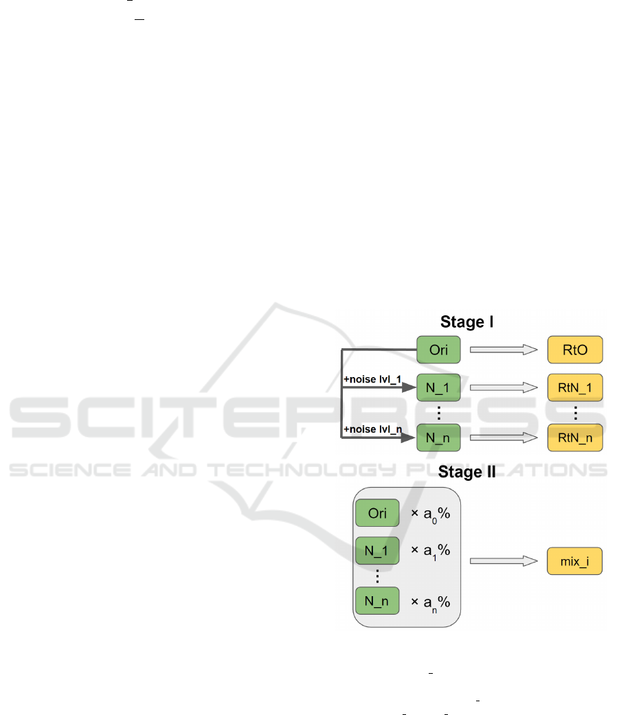
3 METHODOLOGY
We propose a two-stage noise training methodology
as shown in Fig. 2. It improves the robustness of a
CNN model regarding noise resilience when process-
ing jobs such as image classification. Two stages are
Stage I: single-noise training and Stage II: mix-noise
training, or single training and mix training for sim-
plicity. In Stage I, we first construct n noisy sets by
adding n levels of noise to the original training data
and obtain n + 1 sets for training purpose. Then we
train the CNN model on each set and derive n + 1 re-
trained models including one trained on original data
and n single-noise-trained, or single-trained models.
In Stage II, we mix all n + 1 training sets at a propor-
tion of (a
0
%, a
1
%, . . . , a
n
%), where
∑
n
i=0
a
i
= 100.
Then, we train the CNN model on mix training sets
with different proportions. The mix-noise-trained, or
mix-trained model with the best performance is se-
lected as the final outcome of our methodology.
Figure 2: Two-stage noise training methodology: Training
sets and models are denoted using green and yellow chunks
respectively. “Ori/N x” stands for a training set that con-
tains original/level-x noisy data. “RtO” stands for a model
that is Retrained on Ori. “RtN x” stands for a model that is
Retrained on N x. “mix i” is a mix-trained model.
Here, we provide some empirical selections of
aforementioned parameters in the two-stage noise
training methodology. Generating noisy data is one
of the most significant steps as all the noise-trained
models rely on it. The selections for synthetic noise
range and granularity are critical. Intuitively, the
lower bound of noise level is 0, thus noise-free or the
original high-quality image. The upper bound should
KDIR 2022 - 14th International Conference on Knowledge Discovery and Information Retrieval
86

not be the maximum value of the parameters in the
noise-generating function because an image is barely
informative or useful when the noise is extremely in-
tense. In ultrasound imaging scenario, an ultrasound
machine will be recognized as a failure if it produces
noise-dominating ultrasound images. Fixing the ma-
chine would be the top priority instead of digging in-
formation from barely informative images.
We add speckle noise using “imnoise()” in MAT-
LAB. This function is widely used to generate an ar-
tificial noisy image in academic area. The noise in-
tensity is determined by the specified variance. In our
experience, 0.1 is a reasonable upper bound and 0.02
is an appropriate step size. If the granularity is finer,
there is not much difference between two consecutive
noise levels, which introduces redundant information
when doing comparison and analysis. In our experi-
ment, we set the range of speckle noise variance to be
[0, 0.1] at a step size of 0.02, thus five noisy sets are
generated based on the original set.
As there are six models in Stage I, we pick the
top three based on the performance on test sets.
An all-round comparison can be designed depend-
ing on the specific requirements. For example, if
the future images are expected to be less noisy, the
model’s classification performance on sparsely noisy
images should be stressed during the comparison pro-
cess. Then we mix the corresponding training sets
at multiple proportion combinations. Tested propor-
tion choices are (20%, 40%, 40%), (25%, 50%, 25%),
(33%, 33%, 33%) and (40%, 40%, 20%). The propor-
tion of the rest uncollected sets is 0%, hence is omit-
ted for simplicity. The best mix-trained model will be
selected as the final output of this methodology after
comprehensive comparisons.
4 DATASETS AND CNN MODELS
4.1 Dataset Preparation
In our experiments, we mainly work on two public
breast ultrasound image datasets: Breast Ultrasound
Images Dataset (BUSI) (Al-Dhabyani et al., 2020)
and MT small (Badawy et al., 2021). BUSI includes
breast ultrasound images among women between 25
and 75 years old. All images were acquired using
LOGIQ E9 ultrasound and LOGIQ E9 Agile ultra-
sound system by Baheya Hospital, Cairo, Egypt in
2018. It has three classes: benign, malignant and nor-
mal. The sample size of each class is 487, 210 and
133. MT small is a modest dataset that contains 200
images for each class of benign and malignant breast
cancer ultrasound images.
We drop the samples of normal class in BUSI as
the main purpose of the experiments is to determine
whether the nodule is benign or malignant. We as-
sume the presence of a nodule. Moreover, we trim
both datasets by removing samples with on-image
segmentation squares and annotations. This ensures
the training data do not have uncommon features that
distract the model from convergence. Finally, the
trimmed BUSI contains 335 benign and 184 malig-
nant sample images, and the trimmed MT small con-
tains 187 benign and 179 malignant sample images.
The arrangement details of two datasets are pro-
vided in Table 1. BUSI is selected for training pur-
pose because it contains more sample images. As the
malignant sample size (184) is much smaller than be-
nign sample size (335), it affects both convergence
during the training phase and generalization of a
model on the test set (Buda et al., 2018).
In binary classification scenario, class imbalance
problem is more detrimental and the output may al-
ways be the majority class. To address this issue, un-
dersampling and oversampling are two common mea-
sures. Oversampling is widely used and proven to
be robust as mentioned in (Ling and Li, 1998). It is
also justified that oversampling outperforms all other
tested measures with respect to multi-class receiver
operating characteristic curve (ROC AUC) in (Buda
et al., 2018). Moreover, since both the majority and
minority class sample sizes are very small, oversam-
pling is preferred.
It is mentioned in (Buda et al., 2018) that sim-
ply replicates randomly selected samples in the minor
class is an effective oversampling method. But it may
lead to overfitting. Therefore, we randomly select
sample images in malignant class and crop them as
new samples to avoid potential overfitting issue. The
region of interest is ensured to be present in new sam-
ple images. Moreover, a validation set that contains
no oversampling samples is carefully constructed to
mitigate the overfitting risk.
Reasons why other data augmentation methods
are not adopted are 1) they are equivalent or similar
to cropping; and 2) they do not simulate a properly
acquired ultrasound image. For example, as the pre-
processing before feeding the image to a CNN for-
mats the input image into the same shape, scaling
and translation are very similar to cropping. Rota-
tion and flipping may not simulate a proper ultra-
sound image because patients are always required to
keep an upright position when taking the ultrasound
image. Brightness and saturation change may indi-
cate a technical issue with the ultrasound transducer
probe. Therefore, we adopt cropping as the augmen-
tation method here. Two classes have the same size
An Effective Two-stage Noise Training Methodology for Classification of Breast Ultrasound Images
87

(335) after oversampling. They are further divided
into a training set and a validation set at the propor-
tion of 80% and 20% respectively. It is ensured that
the dataset for validation does not contain any over-
sampling samples.
Based on the balanced original dataset, we add
five levels of speckle noise using “imnoise()” in MAT-
LAB. The noise variance is set to 0.02, 0.04, 0.06,
0.08 and 0.1 for the single-noise-training process in
Stage I. These five BUSI dataset noisy variants are
named as BUSI SPE 002, BUSI SPE 004 etc. With-
out causing a confusion, “BUSI ” is omitted for sim-
plicity. To determine the best three single-trained
models, we compare their classification performance
on test sets. Due to the lack of public breast ultra-
sound image data, we take the whole trimmed BUSI
as a test set, together with the trimmed MT small.
This is a very controversial data usage choice be-
cause high similarity between training and test sets
enables models to be more optimal than they really
are. However, the main focus of this work is to ex-
plore the potential performance gain by applying the
proposed two-stage noise training methodology. The
effectiveness of the proposed methodology can be jus-
tified if the over-optimal noise-trained models outper-
form the over-optimal normally trained models, based
on the fact that all of these models are trained and
tested on the same datasets or their noisy variants. In
addition, extreme medical data shortage is undeniable
and cannot be easily solved in the near future. This
decision on data usage is hard and choiceless. Each
of the two test sets, BUSI and MT small, also has five
noisy variants by adding five levels of speckle noise.
To decrease the shortcoming of this data usage,
we comprehensively compare the performance on
two test sets. When they conflict, the test perfor-
mance on MT small plays a more important role
in model ranking. With three Stage I winners, we
construct Stage II training and validation sets from
single-noise sets in Stage I with multiple mix propor-
tion options: (20%, 40%, 40%), (25%, 50%, 25%),
(33%, 33%, 33%) and (40%, 40%, 20%). These four
mixed variant datasets are named as SPE 204040,
SPE 255025 etc. The order of the corresponding
single-noise set is randomly decided because it is of-
ten the case that no model is strictly better than an-
other. In our experiment, the corresponding single-
noise sets are in the ascending noise intensity order.
The same test sets are used to analyze the perfor-
mance of mix-trained models on images at each noise
intensity level.
In conclusion, there are six Stage I train-
ing/validation sets, four Stage II train/validation sets
and twelve test sets for both stages.
Table 1: Details of all the datasets: The values of i
are {1, 2} as there are two stages. Two groups of set
names are: Group 1: {Original, SPE 002, SPE 004,
SPE 006, SPE 008, SPE 010}, Group 2: {SPE 204040,
SPE 255025, SPE 333333, SPE 404020}. B and M in
“Sample Size” stand for benign and malignant respectively.
Purpose
Initial
Dataset
Dataset
Name
Sample Size
Stage i
Train
BUSI Group i
B: 268
M: 268
Stage i
Val
B: 67
M: 67
Test
BUSI
Group 1
B: 335
M: 184
MT small
B: 187
M: 179
4.2 CNN Models
Previous researchers have done ample experiments
on breast ultrasound image classification with CNNs.
Several of them are proved to be very effective and
used as foundations for further studies. They include
AlexNet (Krizhevsky et al., 2012), ResNet (He et al.,
2016) and VGG (Simonyan and Zisserman, 2014).
Therefore, we select four CNN models in our experi-
ment. They are AlexNet, ResNet-18, ResNet-50 and
VGG16. As the pretrained models were trained on
ImageNet (Deng et al., 2009), we replace the out-
put dimension of the last fully-connected layer from
1, 000 to 2 for transfer learning in our methodology.
Since the sample size of our whole training set
(536) is far from comparable to that of ImageNet
(≥ 1.2 million) and medical images are not stressed
in ImageNet, feature extraction of our training data
could be a huge obstacle. Ayana, Gelan, et al.
proposed a multistage transfer learning strategy in
(Ayana et al., 2022) that first fine tunes the pretrained
model with large amount of cancer cell line images,
which can be easily acquired. Then they fine tune the
intermediate model with limited-amount breast can-
cer images to overcome the training data shortage is-
sue and improve the classification performance. We
overlook the shortage issue for now as the main pur-
pose of this work is to show the performance improve-
ment brought by noise training even with very limited
amount of training data.
All the retrained models during our two-stage
noise training methodology are listed in Table 2. In
Stage I, six retrained models, including one trained on
original data and five single-trained models, are gen-
erated by fine tuning the pretrained model. Four mix-
trained models in Stage II are also fine-tuned based
on the pretrained model and trained on mix datasets.
KDIR 2022 - 14th International Conference on Knowledge Discovery and Information Retrieval
88

Table 2: The values of x are {002, 004, 006, 008, 010}. The
values of y are {204040, 255025, 333333, 404020}.
.
Stage CNN Training Set Model
I
AlexNet
ResNet-18/50
VGG16
Original RtO
SPE x RtN x
II SPE y mix y
5 EXPERIMENTS AND RESULTS
In this section, we discuss the performance metrics to
rank models and briefly introduce the implementation
in each stage. The source code of our experiments is
public through GitHub
4
for other researchers to repro-
duce the results and carry out further studies. We also
provide detailed model ranking comments and perfor-
mance analysis of highlighted models in this section.
5.1 Performance Metrics
The performance metrics used in this study are accu-
racy, specificity, sensitivity and F1 score. True/False
indicates the nodule is cancerous/non-cancerous. In
the following equations, TP/TN and FP/FN stand for
true positive/negative and false positive/negative.
Accuracy given by Equation 4 is the proportion of
correct predictions over all types of predictions.
Accuracy(%) =
T P + T N
T P + T N + FP + FN
(4)
Specificity given by Equation 5 is the proportion
of predictions that if a nodule is benign, it is classified
as false.
Speci f icity(%) =
T N
T N + FP
(5)
Sensitivity given by Equation 6 is the proportion
of predictions that if a nodule is malignant, it is clas-
sified as true.
Sensitivity(%) =
T P
T P + FN
(6)
F1 score given by Equation 7 is the harmonic
mean of precision and recall (Taha and Hanbury,
2015). Recall is equivalent to sensitivity and preci-
sion is defined as
T P
T P+F P
. It describes the reliability
of a positive prediction.
F1(%) =
T P
T P +
1
2
(FP + FN)
(7)
Among all four measurements, we rank the prior-
ity as sensitivity, F1 score, accuracy and specificity.
4
https://github.com/YimingBian/Speckle noise IC
When a nodule is benign but tested otherwise, the
patient could have a second check if the classifica-
tion is wrong. The probability of multiple consecutive
wrong classification is significantly low. On the con-
trary, if the nodule is malignant and the result shows
different, it is fatal because it does not raise attention.
We view it as the most critical principle that if a nod-
ule is malignant, the model outputs true, thus TP and
FN are more emphasized. Therefore, sensitivity is the
most significant while specificity is the least.
5.2 Stage I
In Stage I, we fine tune the pretrained model on six
training sets. We obtain RtO and five single-trained
RtN models. We then analyze their performance in
four aspects based on the test results on both BUSI
and MT small test sets. Here are two basic principles
during comparisons of our experiments:
1) better performance on sparse noise test sets val-
ues more than that on intense noise test sets; and
2) higher sensitivity is more important than other
metrics, especially specificity.
For the first point, if the future images are ex-
pected to have higher noise intensity due to, for in-
stance, limitations of hardware, then models with
better performance on intense noise images are pre-
ferred. The model selection is flexible and depends
on the specific requirements. Here, we assume most
of the future input images have sparse speckle noise.
According to the principles, best three models for
each CNN in Stage I are selected after comprehensive
comparisons as shown in Table 3 and 4. We use a
check mark to note the model with the best perfor-
mance in each metric. Specific performance num-
bers can not be provided here because it is a three-
dimension data. For example, the sensitivity cell of
AlexNet model RtO has six numbers behind: 82.84%,
78.03%, 74.89%, 70.8%, 66.42% and 65.31%. Each
is the sensitivity value of the AlexNet RtO model on
the original BUSI test set and its five noisy variant
datasets. Therefore, we provide all the performance
data in the GitHub repository.
Some models have a good performance in
sensitivity while perform poorly in other met-
rics, such as RtN 010 alexnet, RtN 008 resnet18
and RtN 006 vgg16 on BUSI, and RtN 010 alexnet,
RtO resnet18, RtN 008 resnet18, RtN 010 resnet50
and RtN 006 vgg16 on MT small. They are replaced
by the one which has comparable sensitivity and
much better performance in other metrics.
An Effective Two-stage Noise Training Methodology for Classification of Breast Ultrasound Images
89

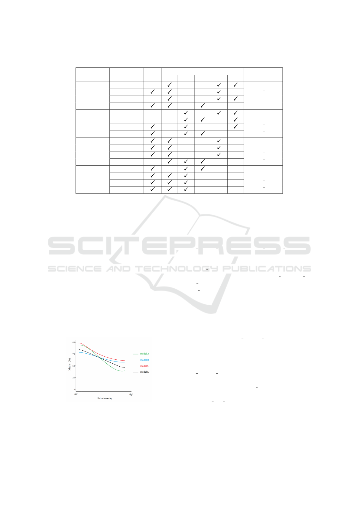
Table 3: Best model selections in Stage I based on their performance on BUSI test sets.
CNN Metric RtO
RtN
Best Models
002 004 006 008 010
AlexNet
Sensitivity
RtN 002
RtN 008
RtN 010
F1 score
Accuracy
Specificity
ResNet-18
Sensitivity
RtO
RtN 004
RtN 010
F1 score
Accuracy
Specificity
ResNet-50
Sensitivity
RtO
RtN 002
RtN 008
F1 score
Accuracy
Specificity
VGG16
Sensitivity
RtO
RtN 002
RtN 004
F1 score
Accuracy
Specificity
5.3 Stage II
With the best models from Stage I, we construct train-
ing and validation sets by combining the correspond-
ing Stage I training sets at certain mix proportions.
Tuning the mix proportion depends on the behavior
of Stage I models. The expectation of mix training
is shown in Fig. 3, model A outperforms model B
when noise intensity is low and otherwise when noise
intensity is high. We would like to mix both training
sets so that the new model obtains the most advan-
tages of both model A and B, and achieve an ideal
performance curve as model C. The bottom line of a
mix-trained model is shown as model D, which has
a mediocre performance compared to model A and B
but demonstrates better capability of noise resilience.
If a mix-trained model performs worse than this bot-
tom line model, the mix-training is a failure and the
corresponding mix proportion should be eliminated.
Figure 3: Mix-training Expectations.
In our experiment, mix proportion options are
(20%, 40%, 40%), (25%, 50%, 25%), (33%, 33%,
33%) and (40%, 40%, 20%). Empirically, it is of-
ten the case that at least one of them generates a
mix-trained model that has a close-to-optimal per-
formance. We comprehensively compare four mix-
trained models following the same rules and de-
termine the best mix-trained model for each CNN.
They are mix 204040 alexnet, mix 404020 resnet18,
mix 333333 resnet50 and mix 404020 vgg16. To
show the mix-training performance gain, we compare
them with the top three models in Stage I on BUSI
and MT small. The performance comparisons among
the best three models in Stage I (RtN 002, RtN 006,
RtN 008) and the best mix-trained model in Stage II
(mix 204040) of AlexNet is provided in Table 5. The
full performance numbers are available on GitHub.
We plot the performance curves of all the best models
in each stage for all CNNs in Fig. 4 and 5.
In all test scenarios, the mix-trained model has
a more stable performance curve with limited fluc-
tuation compared to single-trained models. One
good example is mix 204040 alexnet on both test
sets. It also achieves close-to-optimal performance
curve on BUSI test sets as explained in Fig. 3.
All VGG16 models share a stable and equally
good performance in both test scenarios. However,
mix 333333 resnet50 performs worse than single-
trained models in most scenarios on BUSI but has a
decent performance on MT small test sets. There-
fore, all four mix proportions failed. On the other
hand, RtN 008 resnet50 champions in most test sce-
narios with a stable and good performance such as
the sensitivity on each BUSI and MT small test sets
are {98.22%, 96.09%, 95.11%, 94.65%, 95.68%,
93.12%} and {99.22%, 96.86%, 96.75%, 97.96%,
KDIR 2022 - 14th International Conference on Knowledge Discovery and Information Retrieval
90

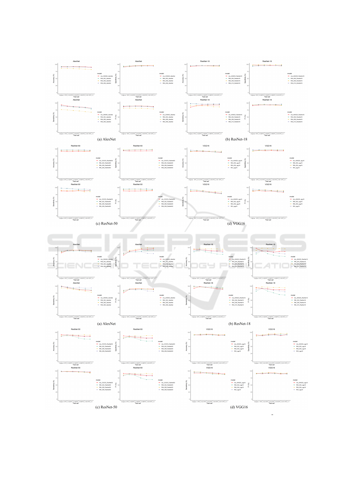
Figure 4: Best single-trained models (Stage I) vs. the best mix-trained model (Stage II) on BUSI.
Figure 5: Best single-trained models (Stage I) vs. the best mix-trained model (Stage II) on MT small.
An Effective Two-stage Noise Training Methodology for Classification of Breast Ultrasound Images
91

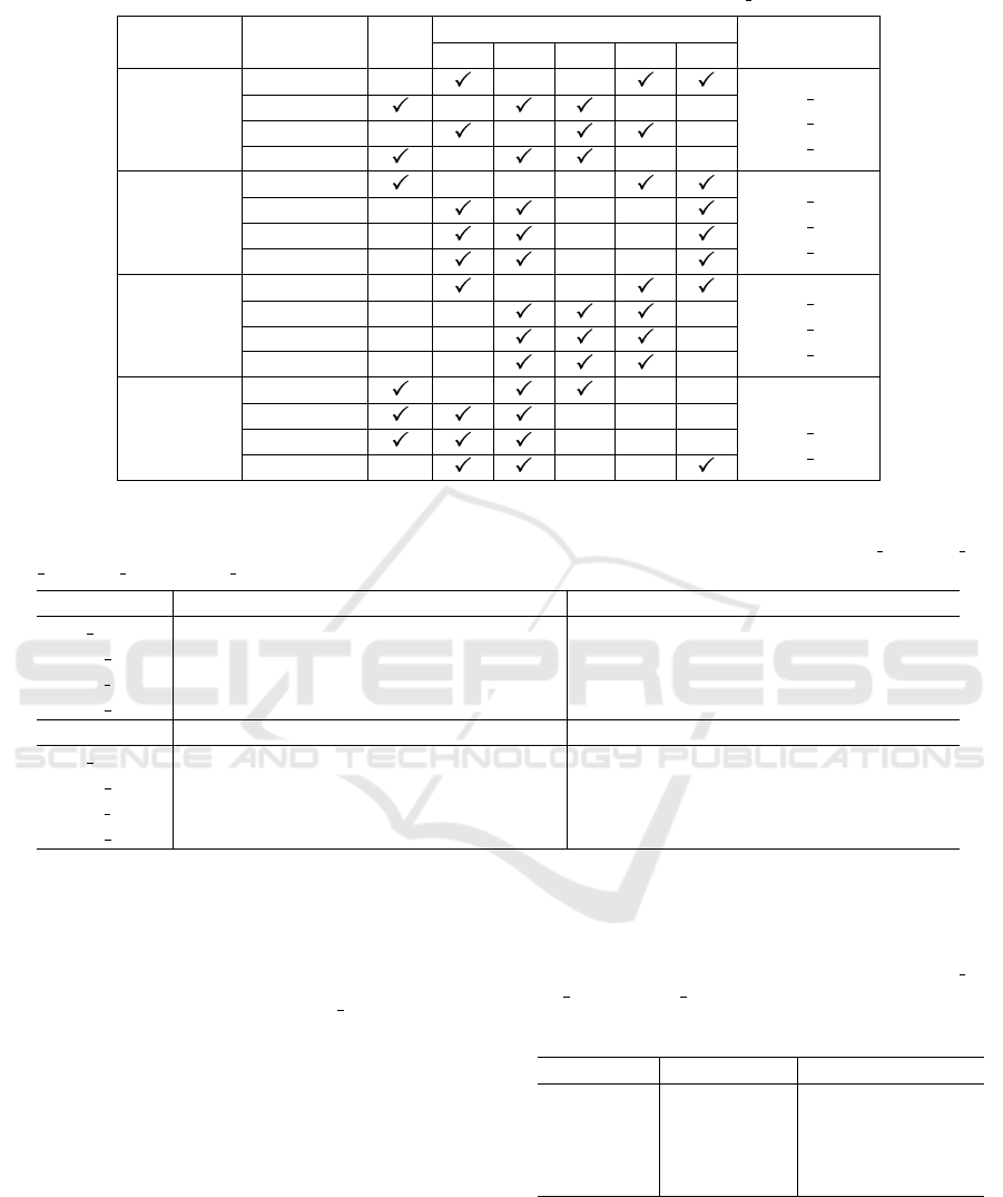
Table 4: Best model selections in Stage I based on their performance on MT small test sets.
CNN Metric RtO
RtN
Best Models
002 004 006 008 010
AlexNet
Sensitivity
RtN 002
RtN 006
RtN 008
F1 score
Accuracy
Specificity
ResNet-18
Sensitivity
RtN 004
RtN 006
RtN 010
F1 score
Accuracy
Specificity
ResNet-50
Sensitivity
RtN 002
RtN 006
RtN 008
F1 score
Accuracy
Specificity
VGG16
Sensitivity
RtO
RtN 002
RtN 004
F1 score
Accuracy
Specificity
Table 5: The performance numbers of the best AlexNet models in each stage on original BUSI and its five noisy variant
test sets: Under the metric cell, the six numbers in a row indicate the model’s performance on Original, SPE 002, SPE 004,
SPE 006, SPE 008 and SPE 010 variant of BUSI test set, respectively. The percent sign is omitted due to the width limit.
Model Sensitivity F1 score
mix 204040 93.3 89.1 87.2 86.0 84.4 81.7 87.7 88.9 89.5 89.4 88.7 87.4
RtN 002 90.1 88.0 85.9 84.1 82.9 78.8 89.4 89.7 89.1 88.8 88.1 86.0
RtN 006 76.6 76.6 73.3 71.9 69.3 67.4 81.2 81.7 81.5 80.9 80.2 78.9
RtN 008 89.5 87.8 87.7 86.1 84.7 81.7 86.0 86.6 88.2 86.6 87.1 85.3
Model Accuracy Specificity
mix 204040 91.8 92.1 92.3 92.1 91.6 90.4 91.0 93.8 95.4 96.0 96.2 96.4
RtN 002 92.5 92.5 92.0 91.6 91.0 89.1 93.8 95.1 95.7 96.5 96.5 96.7
RtN 006 85.8 85.8 85.2 84.5 83.3 82.0 92.0 93.4 94.8 95.1 96.6 96.5
RtN 008 90.4 90.6 91.6 90.4 90.6 89.1 90.9 92.1 93.7 92.8 94.2 93.7
96.27%, 97.69%}. It indicates that Stage II is some-
times redundant when one of the best models in Stage
I achieves very decent performance. One abnor-
mal phenomenon is the poor performance of single-
trained ResNet-18 models on the Mt small Original
test set. Our explanation is that some random process
in Stage I, such as random data sampling, costs the
single-trained model missing benign nodule features.
In Table 6, we provide an empirical training
scheme that generates a noise-trained model with the
best performance for each backbone CNN.
Table 6: The training scheme for each backbone CNN: The
training set is constructed by mixing the noise sets using
the empirical proportion choice provided. For example, for
AlexNet, the training set is developed by mixing SPE 002,
SPE 006 and SPE 008 at a proportion of 20%, 40% and
40%. “000” in Noise Set(s) column indicates the original
data without adding synthetic noise.
Backbone Noise Set(s) Mix Proportion
AlexNet 002,006,008 (20%, 40%, 40%)
ResNet-18 004,006,010 (40%, 40%, 20%)
ResNet-50 008 NA
VGG16 000,002,004 (40%, 40%, 20%)
KDIR 2022 - 14th International Conference on Knowledge Discovery and Information Retrieval
92

6 CONCLUSIONS
In this study, we explore the impact of noisy data
training on noisy data classification and propose a
systematic two-stage noise training methodology. We
mitigate the medical data shortage issue and over-
come class imbalance problem by data augmenta-
tion and oversampling. We comprehensively com-
pare the noise-trained models of three popular back-
bone CNNs in ultrasound image classification field
and provide empirical training scheme for four tested
CNNs. The conclusions regarding the proposed two-
stage training methodology are as follows.
• The mix-trained model always has a more stable
performance curve regardless the noise intensity.
Thus, it is more resilient to speckle noise.
• The performance curve of a mix-trained model
depends on the mix proportion of training sets cor-
responding to single-trained models in Stage I. A
bad mix proportion choice may result in a disas-
trous performance curve.
• If a single-trained model in Stage I has an all-
round decent performance, Stage II may be re-
dundant, especially when other selected single-
trained models perform much worse.
We are interested in flawed medical image pro-
cessing such as breast ultrasound images with speckle
noise because if enough information can be extracted
from a low-quality medical image and useful conclu-
sions can be developed, it would benefit more people
with accessible and reliable medical advice. For fu-
ture research, we plan to expand our work to other
cancer types such as liver cancer, lung adenocarci-
noma etc. Shortage of data is still the biggest chal-
lenge and we also plan to explore CNN architectures
that generalize well on small training datasets.
ACKNOWLEDGEMENTS
The research reported in this paper is partially sup-
ported by the Philip and Virginia Sproul Professor-
ship at Iowa State University and by the HPC@ISU
equipment mostly purchased through funding pro-
vided by the NSF grants numbers MRI1726447 and
MRI2018594.
REFERENCES
Al-Dhabyani, W., Gomaa, M., Khaled, H., and Fahmy, A.
(2020). Dataset of breast ultrasound images. Data in
brief, 28:104863.
Al-Haija, Q. A. and Adebanjo, A. (2020). Breast cancer
diagnosis in histopathological images using resnet-50
convolutional neural network. In 2020 IEEE Interna-
tional IOT, Electronics and Mechatronics Conference
(IEMTRONICS), pages 1–7. IEEE.
Albashish, D., Al-Sayyed, R., Abdullah, A., Ryalat, M. H.,
and Almansour, N. A. (2021). Deep cnn model based
on vgg16 for breast cancer classification. In 2021
International Conference on Information Technology
(ICIT), pages 805–810. IEEE.
Ayana, G., Park, J., Jeong, J.-W., and Choe, S.-w. (2022).
A novel multistage transfer learning for ultrasound
breast cancer image classification. Diagnostics,
12(1):135.
Badawy, S. M., Mohamed, A. E.-N. A., Hefnawy, A. A.,
Zidan, H. E., GadAllah, M. T., and El-Banby, G. M.
(2021). Automatic semantic segmentation of breast
tumors in ultrasound images based on combining
fuzzy logic and deep learning—a feasibility study.
PloS one, 16(5):e0251899.
Bhateja, V., Srivastava, A., Singh, G., and Singh, J. (2014).
A modified speckle suppression algorithm for breast
ultrasound images using directional filters. In ICT and
Critical Infrastructure: Proceedings of the 48th An-
nual Convention of Computer Society of India-Vol II,
pages 219–226. Springer.
Buda, M., Maki, A., and Mazurowski, M. A. (2018).
A systematic study of the class imbalance problem
in convolutional neural networks. Neural networks,
106:249–259.
Chang, Y., Yan, L., Chen, M., Fang, H., and Zhong,
S. (2019). Two-stage convolutional neural network
for medical noise removal via image decomposition.
IEEE Transactions on Instrumentation and Measure-
ment, 69(6):2707–2721.
Daoud, M. I., Abdel-Rahman, S., and Alazrai, R. (2019).
Breast ultrasound image classification using a pre-
trained convolutional neural network. In 2019 15th
International Conference on Signal-Image Technol-
ogy & Internet-Based Systems (SITIS), pages 167–
171. IEEE.
Deng, J., Dong, W., Socher, R., Li, L.-J., Li, K., and Fei-
Fei, L. (2009). Imagenet: A large-scale hierarchical
image database. In 2009 IEEE conference on com-
puter vision and pattern recognition, pages 248–255.
Ieee.
Dodge, S. and Karam, L. (2016). Understanding how image
quality affects deep neural networks. In 2016 eighth
international conference on quality of multimedia ex-
perience (QoMEX), pages 1–6. IEEE.
Forouzanfar, M. and Abrishami-Moghaddam, H. (2011).
Ultrasound speckle reduction in the complex wavelet
domain.
Hadad, O., Bakalo, R., Ben-Ari, R., Hashoul, S., and
Amit, G. (2017). Classification of breast lesions us-
ing cross-modal deep learning. In 2017 IEEE 14th In-
ternational Symposium on Biomedical Imaging (ISBI
2017), pages 109–112. IEEE.
He, K., Zhang, X., Ren, S., and Sun, J. (2016). Deep resid-
ual learning for image recognition. In Proceedings of
An Effective Two-stage Noise Training Methodology for Classification of Breast Ultrasound Images
93

the IEEE conference on computer vision and pattern
recognition, pages 770–778.
Jahangeer, G. S. B. and Rajkumar, T. D. (2021). Early
detection of breast cancer using hybrid of series net-
work and vgg-16. Multimedia Tools and Applications,
80(5):7853–7886.
Jiang, Y., Chen, L., Zhang, H., and Xiao, X. (2019).
Breast cancer histopathological image classification
using convolutional neural networks with small se-
resnet module. PloS one, 14(3):e0214587.
Kim, H. E., Cosa-Linan, A., Santhanam, N., Jannesari, M.,
Maros, M. E., and Ganslandt, T. (2022). Transfer
learning for medical image classification: a literature
review. BMC medical imaging, 22(1):1–13.
Krizhevsky, A., Sutskever, I., and Hinton, G. E. (2012). Im-
agenet classification with deep convolutional neural
networks. Advances in neural information processing
systems, 25.
LeCun, Y., Bengio, Y., and Hinton, G. (2015). Deep learn-
ing. nature, 521(7553):436–444.
Li, X., Wang, Y., Zhao, Y., and Wei, Y. (2022). Fast speckle
noise suppression algorithm in breast ultrasound im-
age using three-dimensional deep learning. Frontiers
in Physiology, page 698.
Ling, C. X. and Li, C. (1998). Data mining for direct mar-
keting: Problems and solutions. In Kdd, volume 98,
pages 73–79.
Liu, S., Wang, Y., Yang, X., Lei, B., Liu, L., Li, S. X., Ni,
D., and Wang, T. (2019). Deep learning in medical
ultrasound analysis: a review. Engineering, 5(2):261–
275.
Masud, M., Hossain, M. S., Alhumyani, H., Alshamrani,
S. S., Cheikhrouhou, O., Ibrahim, S., Muhammad, G.,
Rashed, A. E. E., and Gupta, B. (2021). Pre-trained
convolutional neural networks for breast cancer de-
tection using ultrasound images. ACM Transactions
on Internet Technology (TOIT), 21(4):1–17.
Moon, W. K., Lee, Y.-W., Ke, H.-H., Lee, S. H., Huang, C.-
S., and Chang, R.-F. (2020). Computer-aided diagno-
sis of breast ultrasound images using ensemble learn-
ing from convolutional neural networks. Computer
methods and programs in biomedicine, 190:105361.
Nawaz, W., Ahmed, S., Tahir, A., and Khan, H. A. (2018).
Classification of breast cancer histology images using
alexnet. In International conference image analysis
and recognition, pages 869–876. Springer.
Russakovsky, O., Deng, J., Su, H., Krause, J., Satheesh, S.,
Ma, S., Huang, Z., Karpathy, A., Khosla, A., Bern-
stein, M., et al. (2015). Imagenet large scale visual
recognition challenge. International journal of com-
puter vision, 115(3):211–252.
Sarvamangala, D. and Kulkarni, R. V. (2021). Convolu-
tional neural networks in medical image understand-
ing: a survey. Evolutionary intelligence, pages 1–22.
Simonyan, K. and Zisserman, A. (2014). Very deep con-
volutional networks for large-scale image recognition.
arXiv preprint arXiv:1409.1556.
Taha, A. A. and Hanbury, A. (2015). Metrics for evaluating
3d medical image segmentation: analysis, selection,
and tool. BMC medical imaging, 15(1):1–28.
Virmani, J., Agarwal, R., et al. (2019). Assessment of de-
speckle filtering algorithms for segmentation of breast
tumours from ultrasound images. Biocybernetics and
Biomedical Engineering, 39(1):100–121.
Virmani, J., Agarwal, R., et al. (2020). Deep feature ex-
traction and classification of breast ultrasound images.
Multimedia Tools and Applications, 79(37):27257–
27292.
Wang, Y., Ge, X., Ma, H., Qi, S., Zhang, G., and Yao, Y.
(2021). Deep learning in medical ultrasound image
analysis: a review. IEEE Access, 9:54310–54324.
Yap, M. H., Goyal, M., Osman, F., Mart
´
ı, R., Denton, E.,
Juette, A., and Zwiggelaar, R. (2020). Breast ultra-
sound region of interest detection and lesion localisa-
tion. Artificial Intelligence in Medicine, 107:101880.
Yu, X., Kang, C., Guttery, D. S., Kadry, S., Chen, Y., and
Zhang, Y.-D. (2020). Resnet-scda-50 for breast ab-
normality classification. IEEE/ACM transactions on
computational biology and bioinformatics, 18(1):94–
102.
Yuan, L., Chen, D., Chen, Y.-L., Codella, N., Dai, X., Gao,
J., Hu, H., Huang, X., Li, B., Li, C., et al. (2021). Flo-
rence: A new foundation model for computer vision.
arXiv preprint arXiv:2111.11432.
KDIR 2022 - 14th International Conference on Knowledge Discovery and Information Retrieval
94