Fuzzy and Evidential Contribution to Multilevel Clustering

Martin Cabotte, Pierre-Alexandre H

ebert and

Emilie Poisson-Caillault

Univ. Littoral C

ote d’Opale, LISIC - UR 4491,

Laboratoire d’Informatique Signal et Image de la C

ote d’Opale, F-62100 Calais, France

Keywords:

Multilevel Clustering, Cmeans, Ecm, Split Criterion, Fuzzy Silhouette, Credal Partition, Spectral Clustering.

Abstract:

Clustering algorithms based on split-and-merge concept, divisive or agglomerative process are widely devel-

oped to extract patterns with different shapes, sizes and densities. Here a multilevel approach is considered in

order to characterise general patterns up to ﬁner shapes. This paper focus on the contribution of both fuzzy

and evidential models to build a relevant divisive clustering. Algorithms and both a priori and a posteriori

split criteria are discussed and evaluated. Basic crisp/fuzzy/evidential algorithms are compared to cluster four

datasets within a multilevel approach. Finally, same framework is also applied in embedded spectral space in

order to give an overall comparison.

1 INTRODUCTION

Extracting general behaviours or particular patterns in

data is a common task in various industrial, medical or

environmental applications. K-means and its deriva-

tive algorithms are appreciated for their understand-

ability and explicability of the resulting clusters. They

also are low-cost algorithms on several aspects in-

cluding computation time, development time, energy.

However, in real-life datasets, clusters can have dif-

ferent sizes, densities, shapes (non-convex, related or

thread-like) and ambiguous boundaries. Algorithms

such as K-means don’t perform well on such diverse

datasets, but other clustering approaches such as spec-

tral or multilevel ones suit more. In the past decades,

several multilevel methods were developed in order

to work at different scales depending on the cluster’s

shape.

To deal with non-linearly separable clusters, spec-

tral approaches were proposed, with the aim to trans-

fer data into an embedded spectral space, where the

boundaries between clusters become linear. Numer-

ous clustering problems are based on multiscale prob-

lems, leading to the emergence of multilevel cluster-

ing such as recursive biparted spectral clustering al-

gorithm (Shi and Malik, 2000), spectral hierarchical

clustering HSC (Sanchez-Garcia et al., 2014) or MSC

(Grassi et al., 2019). But computing spectral embed-

ded spaces is time-consuming when applied on nor-

mal/large datasets and can result in not perfectly accu-

https://orcid.org/0000-0001-6564-8762

rate clustering results when noise and ambiguity ap-

pears.

Fuzzy/evidential partition could help to deal with

such noisy datasets. We propose to compare a large

diversity of clustering approaches , on a selection of

possibly noisy datasets: crisp vs fuzzy or evidential,

direct vs multilevel/hierarchical, working in the raw

initial features space or in a spectral embedded space.

This paper is organised as follows: Section 2 pro-

vides multilevel clustering background and a presen-

tation of their split criteria . Section 3 gives the gen-

eral protocol of the methods evaluation and Section

4 analyses the results to highlight beneﬁts and draw-

backs of each method.

2 MULTILEVEL CLUSTERING,

CONCEPT AND PARAMETERS

2.1 Multilevel Approach

A divisive hierarchical clustering approach is used to

build a multilevel structuring of datasets: from global

shapes to ﬁner parts leading to a more precise analysis

of datasets. An illustration of a three-level clustering

is given by Figure 1 (Grassi et al., 2019).

This process can be carried out either from the fea-

tures data or from an embedded space. In both cases,

data would may be ﬁrst normalised if necessary (min-

max scaling for instance).

Cabotte, M., Hébert, P. and Poisson-Caillault, É.

Fuzzy and Evidential Contribution to Multilevel Clustering.

DOI: 10.5220/0011550800003332

In Proceedings of the 14th International Joint Conference on Computational Intelligence (IJCCI 2022), pages 217-224

ISBN: 978-989-758-611-8; ISSN: 2184-2825

217

Figure 1: Multilevel clustering approach.

2.1.1 Multilevel Clustering Framework

Algorithm 1 describes the general MultiLevel Clus-

tering framework (MLC). At each level, for each clus-

tering, the number of clusters K is a posteriori se-

lected by maximising the silhouette criterion of the

K-means algorithm. Then, the sub-dataset is clustered

into K clusters. For each cluster, a split criterion is

computed to assess its quality/compactness (cf. Sec-

tion 2.2). If the criterion doesn’t reach a given thresh-

old, the algorithm restarts the same clustering proce-

dure on it. The whole process stops either when the

maximum level is reached, or when all clusters verify

the split-criterion’s threshold.

Algorithm 1: Multilevel clustering framework.

Require: X data, −1 ≤ chosenT hreshold ≤ 1

Require: MaxLevel ≥ 1, MaxK ≥ 1

clToSplit ← 1 ; NextclToSplit ← {}

treeLabelled ← NU LL

level ← 1

while clToSplit! = {} and level ≤ levelMax do

for X ∈ clToSplit do

← argmax

k∈J2,maxKK

silhouette(clustering(X, k))

clust

← clustering(X , K

)

treeLabelled ← appendTree(clust

)

for Y ∈ clust

criteriaCluster ← ComputeSplitCriterion

if criteriaCluster ≤ chosenT hreshold then

NextclToSplit ← Y ∪ NextclToSplit

end if

end for

level ← level + 1

clToSplit ← NextclToSplit; NextclToSplit ← {}

end while

return treeLabelled

2.1.2 Embedded Space Variant

To relax data shape requirements and to avoid the se-

lection of one suitable partitioning algorithm, each

clustering may be applied in the embedded space

generated by Algorithm 2 (# means cardinal num-

ber). This space consists in the K ﬁrst eigenvectors

of the NJW Laplacian L (Ng and Weiss, 2001), built

from the local kernel gaussian ZP-similarity matrix W

(Zelnik-manor and Perona, 2004). At each level, K is

set to the number of the largest Principal EigenValues

PEV of L.

Algorithm 2: Spectral clustering with K estimation.

Require: X, neighbour, PEV threshold

W ← ZP.similarity.matrix(X ,neighbour)

W ← check.gram.similarityMatrix(W )

L ← compute.laplacian.NJW (W )

K ← #(W $eigenValues > PEVthreshold)

dataSpec ← W$eigenVectors[, 1 : K]

clust

← clustering(dataSpec, K)

return clust

2.2 Stopping Split Criteria

In multilevel clustering, split criterion is an important

feature. This criterion can direct the clustering to-

wards geometry-based clustering, density-based clus-

tering, etc.

The ﬁrst 3 split criteria studied are a priori crite-

ria: they estimate the necessity of a subdivision (with-

out doing it). They assess the homogeneity of the

clusters: low values indicate that they should be sub-

divided. They are:

• The number of wrongly-clustered points named

CardSil, with CardSil = #(silhouette

< 0) <

CardT hreshold, i ∈ cluster C

, as implemented

in the R-package sClust. A threshold set to 0

requires that all points are closer to its cluster’s

neighbours than to points of other clusters.

• The average silhouette of a cluster named Sil =

mean(silhouette

) > SilT hreshold, i ∈ [1;C

]. It

evaluates the overall geometry of a given cluster.

By heuristics, SilThreshold is set to 0.7.

• A fuzzy generalisation of the silhouette criterion:

the Fuzzy Silhouette (Campello and Hruschka,

2006). This fuzzy silhouette (FS) can be in-

terpreted as the silhouette criterion of the clus-

ter cores: it decreases the impact of ambiguous

points.

All the above criteria are a priori split criteria.

If the value of the criterion doesn’t reach a certain

threshold, the clustering of the sub-dataset is com-

puted. We also propose an a posteriori criterion to

deal with fuzzy and evidential approaches:

• The Mass criterion is based on fuzzy or eviden-

tial membership functions. This criterion evalu-

FCTA 2022 - 14th International Conference on Fuzzy Computation Theory and Applications

218

ates the quality of a level clustering by assessing

the non-ambiguity between clusters:

Mass =

∑

k=1

∑

i∈C

)

Indeed, for each point i of the obtained defuzziﬁed

cluster C

, m

) denotes the membership degree

of i to C

: the higher the value, the lower the am-

biguity of its cluster assignment. So, a high Mass

value means that the obtained current clustering is

coherent: it should be kept, and a sub-clustering

level may then be considered. Conversely, a low

value means that the obtained clustering should

not be kept, because of its high ambiguity. In

section 4, 2 variants of this criterion are going to

be compared Mass25 and Mass100: Mass100 de-

notes the original Mass criterion, whereas Mass25

is a more selective variant which averages the

25% lowest membership degrees of each cluster.

3 COMPARISON PROTOCOL

In order to compare approaches, a protocol has been

set up. Considering the variety of algorithms, several

protocols are explained in this section. Furthermore,

parameters settings is also described. Then, quality

criteria are listed followed by there explanation. Fi-

nally, datasets are shown.

3.1 Clustering Algorithms Compared

In order to evaluate fuzzy and evidential contribu-

tion to multilevel clustering, 3 types of algorithms are

compared:

• Direct Algorithms such as K-means, cmeans

(e1071 :: cmeans) as fuzzy algorithm and ecm

(evclust :: ecm) algorithm (Masson and Denœux,

2007) for credal clustering as witness values.

• Agglomerative Algorithms such as high-density

based scanning (dbscan :: hdbscan), agglomera-

tive Ward.d2 clustering (stats :: hclust) and HSC

(sClust :: HierarchicalSC) to compare how well

the fuzzy and evidential multilevel algorithms per-

form well on dense datasets.

• Multilevel Algorithms based on the previous di-

rect algorithms in the initial and spectral cluster-

ing space.

3.2 Overview of the General Protocol

During the process, it is necessary to ensure a good

convergence of all elementary clustering. Thus, each

clustering is computed 10 times, and the best result is

kept, according to its own optimization’s criteria.

Moreover, global clustering approaches are iter-

ated 10 times to make the assessment more robust.

The mean value of each quality criterion is computed

as the ﬁnal result (standard deviation near zero, not

shown).

3.3 Parameter Settings

Let K

∗

be the ground truth number of classes. For di-

rect approach and agglomerative clustering based on

Ward, the K input is set to K

∗

. For others methods, K

is estimated in order to be close to the ground truth.

3.3.1 K Estimation: A ”Fair” Estimation

Method

At each level of multilevel approaches, a number of

clusters K has to be automatically determined. Two

methods are used, depending on the working space

used.

In the initial space, K is determined using silhouette

criterion. Silhouette criterion is computed for each

i ∈ J2, 10K and the i value maximizing the silhouette

criteria is chosen as the optimal K value.

In spectral embedded space, K is set as the num-

ber of prime eigenvalues of Laplacian matrix, which

are higher than a PE V treshold (0.999 by default, i.e.

close to 1-value for numerical error computation)

3.3.2 Split Threshold Estimation: A Supervised

Method

Split threshold has a huge impact in multilevel ap-

proaches that could stop clustering to its ﬁrst level

or result in an over-clustering. In order to avoid an

a priori threshold leading to this kind of aberrant ﬁ-

nal number of clusters, it is rather computed follow-

ing Algorithm 3. The threshold is iteratively tuned,

either by incrementation or decrementation depend-

ing on the split criterion, until the number of clusters

reaches the true number of classes.

3.4 Agglomerative Algorithms: A

Speciﬁc Evaluation Protocol

Two agglomerative methods compared in this paper

have speciﬁc architectures, which require speciﬁc pa-

rameter settings.

- HC -Ward D2 clustering (stats::hclust ) builds a

clustering tree according to within-cluster variance

minimum. Then, dendrogram is cut (stats::cutree) ac-

cording to a K

∗

value.

Fuzzy and Evidential Contribution to Multilevel Clustering

219

- dbscan::hdbscan agglomerates points according to

a core density with a minimum number of points per

cluster (minPts). Two different values of minPts pa-

rameter are considered to reach the K

∗

ground truth:

the closest lower and upper K value.

Algorithm 3: Threshold determination.

Require: data, SplitCriterion, K

∗

if SplitCriterion == mass then

threshold ← 1

else

threshold ← −1

end if

NbFinalCluster ← 0

while NbFinalCluster < K

∗

if SplitCriterion == mass then

threshold ← threshold − 0.05

else

threshold ← threshold + 0.05

end if

cluster ← MLclustering(data, threshold)

NbFinalCluster ← #unique(cluster)

end while

return threshold

3.5 Quality Criteria

To evaluate and compare clustering algorithms, sev-

eral unsupervised quality criteria are computed:

• The Silhouette Score, cluster :: silhouette

achler et al., 2012) measures compactness of

a cluster compared to the minimum inter-cluster

distance. A silhouette score of 1 means that each

clusters is compact and distant whereas a negative

score means that inter-cluster distance are smaller

than intra-cluster distance.

• The Adjusted Rand Index, pd fCluster ::

ad j.rand.index (Azzalini and Menardi, 2013) is

a corrected-for-chance Rand Index. It measures

the ratio of the agreement between the true and

the predicted partitions over the total number of

pairs.

• The non-Overlap, corresponds to a part of the

Rand Index. The non-overlap index measures the

ratio of non-overlapping pairs over the total num-

ber of pairs. A value of 1 means that all points

are affected to non-overlapping clusters (a cluster

included in a class) and that real classes could be

retrieved.

After assigning clusters to classes using major-

ity vote, two adapted supervised quality criteria are

added to catch non representation of one ground truth

class in the obtained clusters and to detect small

shapes:

• Precision*:

∗

∑

i∈J1,K

∗

T P

(T P

+ FP

)

• Recall*:

∗

∑

i∈J1,K

∗

T P

(T P

+ FN

)

With K

∗

the number of classes, the numbers T P: True

positive, FP: False Positive, FN: False Negative and

= 1 if no cluster is assigned in class i, 0 otherwise.

Sometimes, majority vote doesn’t perform well and

small classes are affected to bigger ones. So α term

penalises non represented classes in the standard pre-

cision and recall formula.

3.6 Data Presentation

Considering the diversity of clustering algorithms,

different types of datasets are compared based on their

speciﬁcity. Some datasets favour some algorithms

(e.g, hierarchical algorithms are designed for dense

datasets, fuzzy and evidential algorithms are made to

characterise ambiguity...). Thus, 3 types of datasets

are used in this comparison: two are non ambiguous

and dense datasets, and the last one has ambiguity and

uncertainty. A representation of the 3 datasets can be

seen ﬁgure 2.

• (A) Aggregation (Gionis et al., 2007) is a well-

segmented dataset composed of 7 clusters. In this

seven clusters, two pairs of clusters are connected

by few points, which usually disturbs the clas-

sical hierarchical clustering, such as HDBSCAN

(McInnes et al., 2017) or stats::hclust.

• (B) Coumpound (Zahn, 1971) is a 2-level dataset

composed of 3 clusters that can be divided into 2

clusters. A pair of clusters has the same speciﬁcity

as aggregation dataset (they are connected by few

points). Another pair of clusters is made in a way

that one is included into the other. These two clus-

ters are merged in order to not penalise some clus-

tering algorithms in raw feature space; they can be

easily separated using spectral approaches. The

last pair is a cluster surrounded by a noise cluster.

• (C) 6-Bananas is a dataset built using the function

evclust::bananas (Denœux, 2021). This dataset is

designed for multilevel approaches. Three sets of

bananas are positioned the same way as Coum-

pound dataset. This dataset is made for fuzzy and

evidential clustering according to its non-linear

cut between bananas.

FCTA 2022 - 14th International Conference on Fuzzy Computation Theory and Applications

220

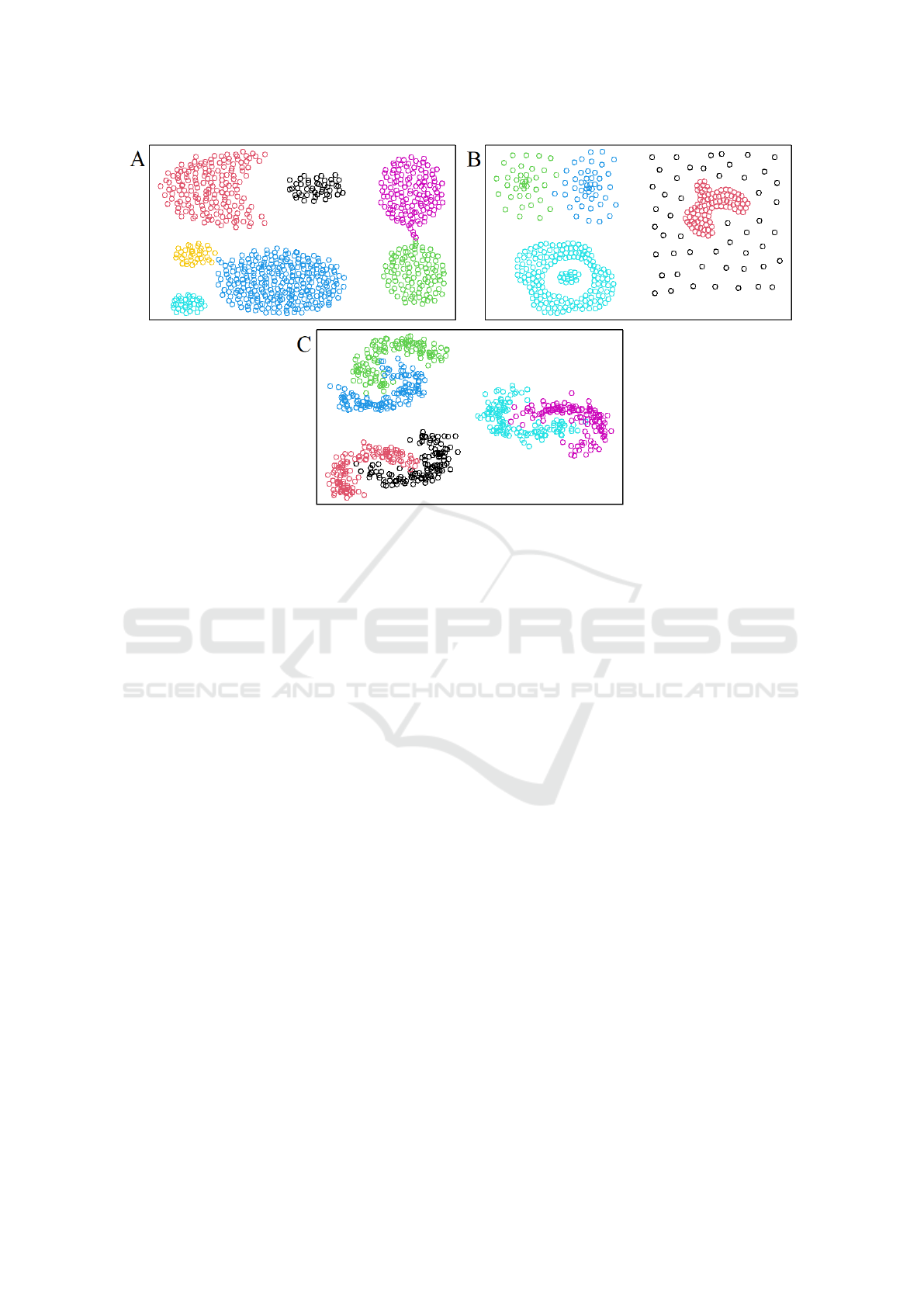
Figure 2: Datasets used with ground truth classes, one color per class - (A) Aggregation - (B) Coumpound - (C) 6-Bananas.

4 RESULTS AND ANALYSIS

In order to understand how well fuzzy and eviden-

tial algorithm perform, the analysis will begin with

datasets where current multilevel approaches perform

well. Finally, a focus on Bananas dataset will be pre-

sented where fuzzy and evidential methods are more

appropriate.

4.1 Aggregation and Coumpound

Dataset Results

Aggregation and Coumpound are ﬁrst clustered in

spectral embedded space (cf. the upper part of Ta-

ble 1). The main quality criterion analysed is ARI,

well-suited to the unsupervised approach.

Compound results of multilevel C-means

(Mass25/Mass100) as well as multilevel K-means

(CardSil) have high ARI scores. A deeper under-

standing of theses values is given in the following

rows. Precision* and Recall* scores show that

multilevel K-means isn’t as efﬁcient as multilevel

C-means. Those lower scores can be primarily

explained by a class disappearance induced by a

lower number of resulting clusters.

This low number of ﬁnal clusters obtained by the

ML K-mean (CardSil) algorithm (cf. ﬁfth row of Ta-

ble 1), can’t be increased because of the architecture

of the split criterion. Indeed, the roughest thresh-

old value is already selected. This highlights a limit

of this split criterion: it may stop sub-clustering too

early, if a cluster appears ”coherent”, despite being

composed of several subclusters.

Aggregation results show that multilevel ECM

(Mass25) perfectly retrieves real classes: its ARI

score almost reaches 1. Multilevel K-means

(Sil), C-means (FS/Mass25/Mass100) and ECM

(FS/Mass100) have a high precision value but over-

cluster the dataset. However, it should be noted that

Mass split-criteria can lead to lower number of clus-

ters than FS/Sil criteria.

In order to challenge a bit more algorithms, clus-

tering is also performed in the initial features space.

According to ARI, Aggregation is the most difﬁcult

dataset for fuzzy and evidential methods. Hierarchi-

cal clustering performs well on this dataset; and mul-

tilevel K-means is the best multilevel algorithm with

only few overlapping pairs (less than 2%) and a good

precision. Coumpound conclusions are slightly dif-

ferent. Multilevel K-means (Sil) results are equal to

C-means (FS) with good precision and non-overlap

values but result in a total of 23 clusters whereas mul-

tilevel C-means (Mass100) and ECM (Mass100) have

better ARI and non-Overlapping scores with half ﬁ-

nal clusters: on this dataset, the resulting clustering is

better using fuzzy and evidential approaches.

To sum up, spectral clustering is improved on

certain datasets using fuzzy/evidential clustering and

is equal on others. The reason is that compact,

dense and distant clusters will still remain in spec-

tral embedded space. But if ambiguity is kept or cre-

Fuzzy and Evidential Contribution to Multilevel Clustering

221

Table 1: Clustering results obtained in embedded spectral space (top section) and raw feature space (bottom section) by:

K-means (KM), C-means (CM), Evidential C-means (ECM), agglomerative Ward.d2 clustering (HC), High Density Based

Scanning (HDBSCAN) with K estimation (lower and upper closest values of K) and all Multilevel variants (ML).

Direct (1) Agglomerative (2) ML KM (3) ML CM (4) ML ECM (5)

KM CM ECM HC HDBSCAN CardSil Sil FS Mass25 Mass100 FS Mass25 Mass100

Embedded spectral space

Coumpound K*=6

ARI 0.49 0.43 0.43 0.51 0.86-0.45 0.81 0.36 0.26 0.85 0.85 0.26 0.58 0.58

NonOverlap 0.92 0.91 0.91 0.92 0.94 0.92 1 1 0.94 0.94 1 0.99 0.94

Precision* 0.7 0.52 0.52 0.7 0.92 0.7 0.99 1 0.94 0.94 0.99 0.97 0.94

Recall* 0.67 0.5 0.5 0.67 0.79-0.78 0.67 0.99 1 0.83 0.83 0.99 0.93 0.83

NbClusters 6* 6* 6* 6* 5-7 4 17 28 7 7 21 14 13

Aggregation K*=7

ARI 0.96 0.95 0.77 0.99 0.99-0.44 0.81 0.33 0.29 0.85 0.29 0.29 0.96 0.45

NonOverlap 1 1 0.99 1 1-0.97 0.93 1 1 0.97 1 1 1 1

Precision* 0.96 0.94 0.77 0.99 0.99-0.96 0.64 0.95 1 0.84 1 1 1 1

Recall* 0.99 0.98 0.85 0.99 1-0.89 0.71 0.99 0.99 0.85 0.99 0.99 0.99 0.99

NbClusters 7* 7* 7* 7* 7-20 5 21 38 14 37 38 8 26

6-Bananas K*=6

ARI 0.65 0.63 0.64 0.66 0.59-0.57 0.57 0.35 0.32 0.55 0.49 0.32 0.41 0.49

NonOverlap 0.95 0.95 0.95 0.95 0.93-0.93 0.83 0.99 0.99 0.88 0.93 0.99 0.98 0.93

Precision* 0.82 0.81 0.82 0.84 0.63- 0.63 0.25 0.92 0.93 0.46 0.68 0.92 0.87 0.67

Recall* 0.82 0.81 0.82 0.83 0.72-0.71 0.5 0.91 0.92 0.61 0.74 0.91 0.85 0.74

NbClusters 6* 6* 6* 6* 6-8 3 23 24 7 13 24 18 13

Feature space

Coumpound with class fusion K*=5

ARI 0.57 0.51 0.48 0.59 0.76 - 0.84 0.5 0.28 0.28 0.45 0.8 0.35 0.47 0.83

NonOverlap 0.94 0.95 0.93 0.94 0.94-0.98 0.74 0.94 0.94 0.79 0.97 0.94 0.79 0.94

Precision* 0.84 0.64 0.63 0.91 0.89-0.94 0.47 0.93 0.93 0.49 0.67 0.92 0.44 0.92

Recall* 0.74 0.6 0.59 0.79 0.76-0.9 0.4 0.8 0.8 0.5 0.7 0.8 0.48 0.8

NbClusters 5* 5* 5* 5* 6-9 2 23 24 6 7 12 6 11

Aggregation K*=7

ARI 0.76 0.74 0.55 0.81 0.81-0.67 0.66 0.56 0.52 0.63 0.59 0.55 0.52 0.52

NonOverlap 0.99 0.99 0.92 1 0.93-0.93 0.98 0.99 0.97 0.93 0.94 0.97 0.95 0.95

Precision* 0.76 0.76 0.47 0.79 0.64-0.64 0.95 0.97 0.79 0.65 0.66 0.76 0.67 0.67

Recall* 0.83 0.83 0.54 0.86 0.71-0.71 0.89 0.93 0.83 0.61 0.7 0.82 0.66 0.66

NbClusters 7* 7* 7* 7* 5-55 14 18 15 13 17 25 14 14

6-Bananas K*=6

ARI 0.57 0.59 0.57 0.67 0.57-0.03 0.57 0.37 0.37 0.54 0.54 0.38 0.49 0.51

NonOverlap 0.94 0.94 0.93 0.94 0.83-0.98 0.83 0.94 0.94 0.96 0.96 0.94 0.96 0.92

Precision* 0.76 0.78 0.79 0.86 0.25-0.92 0.25 0.73 0.73 0.84 0.84 0.72 0.8 0.63

Recall* 0.76 0.78 0.75 0.82 0.5-0.87 0.5 0.81 0.81 0.84 0.84 0.8 0.79 0.72

NbClusters 6* 6* 6* 6* 3-218 3 75 64 10 10 50 14 14

ated while transferring data into spectral embedded

space, fuzzy/evidential methods will improve cluster-

ing thanks to their membership characterisation.

Also, CardSil split criterion shows its limits in raw

features space, because the lowest possible estimated

K is often lower than the ground-truth value. Thus,

ﬁner shapes can’t be retrieved, restraining multilevel

approach.

4.2 A More Difﬁcult Dataset:

6-Bananas

Bananas dataset combines several difﬁculties: cluster

boundaries are non-linear, very close to each other,

ambiguous, and the cluster densities are weak (each

banana has 125 points, ambiguity included). There-

fore, clustering is particularly hard.

Clustering in Spectral Space. The too high con-

nexity between bananas does not allow building a rel-

evant spectral space. But this spectral space causes in

most cases lower ﬁnal number of clusters and homo-

geneous clusters (non-overlap scores are almost equal

to 1).

Clustering in Raw Features Space. Direct meth-

ods with true value of K achieve quite good ARI re-

sults. However, they do not clearly exceed 0.57, the

ARI score obtained by the 2 methods resulting in

K = 3 clusters (pairs of bananas are identiﬁed, but

without a ﬁner division). HC with the true value of K

gives the best clustering with an ARI equal to 0.67 and

only 6% of overlapping pairs of points. HDBSCAN is

not particularly efﬁcient on this dataset. With 3 min-

imum points per cluster (minPts = 3), the algorithm

gives only 3 ﬁnal clusters, and when the minimum

number of points per cluster is decreased to 2 points,

FCTA 2022 - 14th International Conference on Fuzzy Computation Theory and Applications

222

the algorithm gives a total of 218 clusters resulting in

a disastrous ARI.

Multilevel K-means (CardSil), as mentioned

above, stops at the ﬁrst level and only detects the pairs

of bananas.

Then two groups can be identiﬁed:

• the Sil/FS split criterion, which builds more than

50 ﬁnal clusters. This overclustering leads to

weak ARI scores. The crisp multilevel FS K-

means is the worst, with 25 more clusters than

ECM but the same quality criterion values.

• the Mass25 and Mass100 group determines be-

tween 10 and 14 ﬁnal clusters. These split criteria

have higher ARI (0.54 with MC CM) and almost

equal non-overlap scores with less clusters, mean-

ing that they perform better than the Sil/FS ones.

To summarise, fuzzy and evidential approach can

improve multilevel clustering results, in spite of noisy

non-linearly separable clusters. However, on this

dataset, ML variants do not achieve the best ARI

(HC’s score), which can be explained by their higher

number of ﬁnal clusters. But those clusters are very

homogenous (high non-overlap scores).

5 CONCLUSION

In this paper, we have mainly proposed a compari-

son between clustering methods: direct vs multilevel,

then crisp vs fuzzy/evidential. To enhance the fuz-

zy/evidential multilevel algorithms, a new split crite-

rion has also been proposed (Mass a posteriori split

criterion).

Several conclusions were obtained. First, direct

methods may result in a bad structure recognition

due to particular geometry shapes like nested or close

clusters. Agglomerative methods may also be dis-

turbed by connected noisy clusters. This problem

also affects HDBSCAN, despite its ability to cluster

noise. Moreover, the number of clusters obtained by

HDBSCAN can be extremly sensitive to its parameter

minPts on this type of datasets.

An other shortcoming of agglomerative methods,

and spectral clustering as well, is their complexity:

they are not suitable for large datasets because of too

high computing times.

Multilevel approaches like multilevel C-means or

ECM can help to recognize noisy/ambiguous clusters,

what’s more, in a reasonable computing time. On

some datasets, the ﬁnal clustering appears a lot better

than those obtained with direct methods: the ambigu-

ity between clusters may be better processed working

with several levels.

Then the comparison of split-criteria leads to the

conclusion that those based on soft membership de-

grees can limit the over-clustering, with a K-number

closer to the ground truth.

Nevertheless, multilevel approaches based on K-

means and its fuzzy/evidential extensions are clearly

not perfect. In particular, they are based on a delicate

task, the automatic estimation of the cluster number,

which is repeated frequently.Their parameters are es-

timated in order to obtain a ﬁnal number of clusters

close to the known number of classes. Another reason

which may disadvantage multilevel methods, is the

difﬁculty to obtain a fair comparison with other clus-

tering methods, when the ﬁnal number of clusters dif-

fers. Split criteria thresholds were chosen to make this

number closer to the ground-truth, but it often failed:

they tend to overcluster. But, the fuzzy/evidential

approach provides ambiguity information on clusters

that could be used to perform a fusion and retrieve

original classes. The good non-overlapping scores

obtained in the experiments tend to support this idea.

Further works will therefore investigate the char-

acterization of points and clusters ambiguity in fuzzy

and evidential algorithms, in order to improve each

clustering step, and to drive the merger process to

the building of a more coherent ﬁnal clustering tree.

Moreover, such an approach would reduce the com-

puting time, by making the spectral embedding step

useless.

ACKNOWLEDGMENTS

This work is a part of the JERICO-S3 project, funded

by the European Commission’s H2020 Framework

Programme under grant agreement No. 871153.

Project coordinator: Ifremer, France.

REFERENCES

Azzalini, A. and Menardi, G. (2013). Clustering Via Non-

parametric Density Estimation: the R Package pdf-

Cluster.

Campello, R. and Hruschka, E. (2006). A fuzzy extension

of the silhouette width criterion for cluster analysis.

Fuzzy Sets and Systems, 157(21):2858–2875.

Denœux, T. (2021). evclust: An R Package for Evidential

Clustering. Bananas dataset.

Gionis, A., Mannila, H., and Tsaparas, P. (2007). Clus-

tering aggregation. ACM Transactions on Knowledge

Discovery from Data, 1(1):4.

Grassi, K., Poisson Caillault, E., and Lefebvre, A. (2019).

Multilevel spectral clustering for extreme event char-

acterization. In OCEANS 2019 - Marseille. IEEE.

Fuzzy and Evidential Contribution to Multilevel Clustering

223

Masson, M.-H. and Denœux, T. (2007). Algorithme

evidentiel des c-moyennes ecm : Evidential c-means

algorithm. In Rencontres Francophones sur la

Logique Floue et ses Applications (LFA’07), pages

17–24, N

ımes, France, Novembre, 2007.

McInnes, L., Healy, J., and Astels, S. (2017). hdbscan: Hi-

erarchical density based clustering. The Journal of

Open Source Software, 2(11):205.

achler, M., Rousseeuw, P., Struyf, A., Hubert, M., and

Hornik, K. (2012). Cluster: Cluster Analysis Basics

and Extensions, R-CRAN packages.

Ng, A.and Jordan, M. and Weiss, Y. (2001). On Spectral

Clustering: Analysis and an algorithm. In Advances

in Neural Information Processing Systems (NIPS’01),

pages 849–856. MIT Press.

Sanchez-Garcia, J., Fennelly, M., Norris, S., Wright, N.,

Niblo, G., Brodzki, J., and Bialek, J. W. (2014). Hi-

erarchical spectral clustering of power grids. IEEE

Transactions on Power Systems, 29(5):2229–2237.

Shi, J. and Malik, J. (2000). Normalized cuts and image

segmentation. IEEE Trans. Pattern Anal. Mach. In-

tell., 22(8):888–905.

Zahn, C. (1971). Graph-theoretical methods for detecting

and describing gestalt clusters. IEEE Transactions on

Computers, C-20(1):68–86.

Zelnik-manor, L. and Perona, P. (2004). Self-tuning spec-

tral clustering. In Saul, L., Weiss, Y., and Bottou, L.,

editors, Advances in Neural Information Processing

Systems (NIPS’04). MIT Press.

FCTA 2022 - 14th International Conference on Fuzzy Computation Theory and Applications

224