Sample-based Uncertainty Quantification with a Single Deterministic
Neural Network
Takuya Kanazawa and Chetan Gupta
Industrial AI Lab, Hitachi America, Ltd. R&D, Santa Clara, CA, 95054, U.S.A.
Keywords:
Uncertainty Quantification, Ensemble Forecasting, CRPS, Aleatoric Uncertainty, Epistemic Uncertainty,
Energy Score, DISCO Nets.
Abstract:
Development of an accurate, flexible, and numerically efficient uncertainty quantification (UQ) method is
one of fundamental challenges in machine learning. Previously, a UQ method called DISCO Nets has been
proposed (Bouchacourt et al., 2016) that trains a neural network by minimizing the so-called energy score
on training data. This method has shown superior performance on a hand pose estimation task in computer
vision, but it remained unclear whether this method works as nicely for regression on tabular data, and how it
competes with more recent advanced UQ methods such as NGBoost. In this paper, we propose an improved
neural architecture of DISCO Nets that admits a more stable and smooth training. We benchmark this approach
on miscellaneous real-world tabular datasets and confirm that it is competitive with or even superior to standard
UQ baselines. We also provide a new elementary proof for the validity of using the energy score to learn
predictive distributions. Further, we point out that DISCO Nets in its original form ignore epistemic uncertainty
and only capture aleatoric uncertainty. We propose a simple fix to this problem.
1 INTRODUCTION
In real-world applications of artificial intelligence (AI)
and machine learning (ML), it is becoming essential
to estimate uncertainty of predictions made by AI/ML
models. This is especially true in high-stakes areas
such as health care and autonomous driving, where
inadvertent decisions can cause fatal damages. While
traditional methods for uncertainty quantification (UQ)
such as bootstrapping and quantile regression can be
partly applied to modern AI/ML models, the rapid
progress especially in the field of deep neural networks
calls for a development of novel UQ methodologies
(Abdar et al., 2021; Gawlikowski et al., 2021).
In this paper, we revisit a UQ method for neural net-
works (NN) on regression tasks. This method, called
DISCO Nets (DISsimilarity COefficient Networks)
(Bouchacourt et al., 2016), enables us to estimate un-
certainty of a prediction in a fully nonparametric man-
ner by using just a single deterministic NN (see also
(Harakeh and Waslander, 2021; Pacchiardi et al., 2021)
for related studies). Unlike Bayesian NN and Gaussian
processes, DISCO Net does not encounter computa-
tional bottlenecks when it is scaled to a large problem.
In addition, it can model a posterior distribution in
more than one dimension straightforwardly, in contrast
to conventional quantile regression-based methods that
do not trivially generalize to higher dimensions.
Despite its flexibility and versatility, however,
DISCO Net has not gained popularity comparable to
other UQ methods such as Monte Carlo dropout (Gal
and Ghahramani, 2016). There could be multiple rea-
sons for that. First, DISCO Net belongs to a class
of NN called implicit generative networks, which are
generally difficult to train (Tagasovska and Lopez-Paz,
2019). Second, understanding the theoretical underpin-
ning of DISCO Net requires sophisticated mathematics
and statistics of scoring rules of distributions, which
makes the method unfamiliar and less approachable
for data science practitioners in industry. Third, while
it is widely known that there are two types of uncer-
tainty in ML called aleatoric uncertainty and epistemic
uncertainty (Abdar et al., 2021; Gawlikowski et al.,
2021; Hüllermeier and Waegeman, 2021), it is not to-
tally obvious which of these uncertainties is estimated
by DISCO Net. Fourth, DISCO Net has so far been
primarily benchmarked on a limited range of tasks
in computer vision, and evidence of its favorable per-
formance on learning tasks on tabular data has been
missing in the literature, despite abundance of tabular
data in industry.
292
Kanazawa, T. and Gupta, C.
Sample-based Uncertainty Quantification with a Single Deterministic Neural Network.
DOI: 10.5220/0011546800003332
In Proceedings of the 14th International Joint Conference on Computational Intelligence (IJCCI 2022), pages 292-304
ISBN: 978-989-758-611-8; ISSN: 2184-3236
Copyright © 2023 by SCITEPRESS – Science and Technology Publications, Lda. Under CC license (CC BY-NC-ND 4.0)

Figure 1: Left: random data points. Right: the result of
applying DN+ to the same data. Aleatoric uncertainty is
quantified appropriately. See section 5 for more detail.
We wish to address all these points in this paper.
First, we propose an improved NN architecture of
DISCO Net. The original DISCO Net assumed that a
noise vector was simply concatenated to the input vec-
tor before being fed to the NN. However, empirically,
the training of NN with this method is found to be diffi-
cult. The original work (Bouchacourt et al., 2016) has
overcome this difficulty by using a very high ( ∼ 200 )
dimensional noise vector, but it consequently requires
a quite large NN and thus increases the training time.
We rather propose to simply insert an embedding layer
of a noise vector. This trick leads to stable learning
even for a one-dimensional noise vector and boosts
computational efficiency substantially. Second, we
provide a rudimentary analytical proof that training of
NN using the energy score allows to learn the correct
predictive distribution, at least when the batch size in
stochastic gradient descent training is large enough.
We hope this will make DISCO Net more accessible
and trustworthy for practical data scientists. Third,
we numerically verify that DISCO Net misses epis-
temic uncertainty, although it is capable of capturing
aleatoric uncertainty quite well. We propose to use
an oscillatory activation function in DISCO Net to
capture epistemic uncertainty. Fourth, we conduct ex-
tensive numerical experiments to test the effectiveness
of the proposed approach for tabular datasets. We use
10 real-world datasets and show that the UQ capability
of the present approach is competitive with or even
superior to popular baseline methods.
The enhanced DISCO Net approach proposed in
this work will be referred to as DN+ in the remainder
of this paper.
In section 2 we summarize preceding works on
UQ in machine learning. In section 3 we provide
the background of this research, introducing concepts
such as the energy score and CRPS. In section 4 we
review DISCO Nets. Section 5 is about our main
contributions, i.e., improvements on DISCO Nets, dis-
cussions on numerical experiments, and comparison
with baselines. We conclude in section 6. A theoreti-
cal discussion on the validity of UQ training using the
energy score is relegated to the appendix, owing to its
technical nature.
2 RELATED WORK
In a classification problem, the uncertainty of an ML
model may be concisely represented by class proba-
bilities that sum to unity. In contrast, the uncertainty
in regression is more complicated. Many existing UQ
methods for regression calculate only the X % con-
fidence interval, where X ∈ {95,99} are among the
common choices. Although such a single interval esti-
mate is quite useful from a practical point of view, it
lacks detailed information on the shape of the posterior
distribution p(y|x) , where x denotes the input variable
and y the output variable. Classical approaches such
as the Gaussian process regression (Rasmussen and
Williams, 2006) can represent the posterior as a multi-
variate Gaussian distribution, but fails when the noise
is heteroscedastic and is unable to express multimodal
posterior distributions.
A variety of improved UQ methods for deep NN
have been proposed in the literature (Abdar et al., 2021;
Gawlikowski et al., 2021).
1
Pivotal examples include
Bayesian NN (Lampinen and Vehtari, 2001), quantile
regression NN (Cannon, 2011), NN that model Gaus-
sian mixtures (Bishop, 1994), ensembles of NN (Lak-
shminarayanan et al., 2017; Pearce et al., 2020), Monte
Carlo dropout (Gal and Ghahramani, 2016), and direct
UQ approaches (Lahlou et al., 2021). These meth-
ods effectively work to quantify either aleatoric un-
certainty, epistemic uncertainty, or both (Hüllermeier
and Waegeman, 2021). Aleatoric uncertainty repre-
sents inherent stochasticity of the response variable,
whereas epistemic uncertainty comes from limitation
of knowledge and can be decreased by gathering more
data.
Recently, normalizing flows (NF) (Kobyzev et al.,
2021; Papamakarios et al., 2021) have emerged as a
versatile and flexible tool for UQ. NF is a generative
model that uses a composition of multiple differen-
tiable bijective maps modeled by NN to transform a
simple (such as uniform or Gaussian) distribution to
a more complex distribution of real data. Examples
of probabilistic forecast based on NF can be found
in (Sick et al., 2020; Charpentier et al., 2020; Dumas
et al., 2021; Sendera et al., 2021; Jamgochian et al.,
2022; Rittler et al., 2022; März and Kneib, 2022; Ar-
pogaus et al., 2022; Cramer et al., 2022).
1
Here we will focus on work other than DISCO Net
(Bouchacourt et al., 2016; Harakeh and Waslander, 2021;
Pacchiardi et al., 2021) because the latter was discussed in
great detail in Introduction.
Sample-based Uncertainty Quantification with a Single Deterministic Neural Network
293

Ensembles from a single NN (known as implicit
NN ensembles) have been studied in (Huang et al.,
2016; Huang et al., 2017; Tagasovska and Lopez-
Paz, 2019; Maddox et al., 2019; Antoran et al., 2020).
While (Huang et al., 2016; Antoran et al., 2020) pro-
pose a NN with a probabilistic depth, (Huang et al.,
2017; Maddox et al., 2019) suggest to use information
in a stochastic gradient descent trajectory of a single
NN to construct ensembles.
Gradient boosting decision trees are among the
most popular ML models, which often outperform NN
as a point forecaster on benchmark tests with tabu-
lar data. Recently, probabilistic forecasts in gradient
boosting decision trees have been studied in (Duan
et al., 2020; Sprangers et al., 2021; Brophy and Lowd,
2022). While (Duan et al., 2020; Sprangers et al.,
2021) require fitting a parametric distribution (such as
Gaussian or Weibull) to the data, (Brophy and Lowd,
2022) allows to produce a more flexible, nonparamet-
ric distributional forecast.
3 BACKGROUND
3.1 Distance between Probability
Distributions
The discrepancy (distance) between two continuous
probability distributions can be quantified using a va-
riety of metrics such as f -divergences. One of the
popular metrics in machine learning is the maximum
mean discrepancy (MMD) (Gretton et al., 2012)
MMD[F, p,q] := sup
f ∈F
(E
x∼p
[ f (x)] − E
y∼q
[ f (y)]) (1)
where p and q are distributions and F is a class of real-
valued functions f : X → R . When F is a reproducing
kernel Hilbert space, there exists a kernel function
k : X × X → R such that
MMD
2
[F, p,q] = E
x,x
0
∼p
[k(x, x
0
)] − 2E
x∼p,y∼q
[k(x, y)]
+ E
y,y
0
∼q
[k(y, y
0
)]. (2)
MMD has been recently used in deep reinforcement
learning to model the distribution of future returns
(Nguyen-Tang et al., 2021; Zhang et al., 2021).
A closely related quantity that measures the statis-
tical distance between two distributions in Euclidean
space is the so-called energy distance (Szekely, 2003;
Szekely and Rizzo, 2004; Szekely and Rizzo, 2013;
Szekely and Rizzo, 2017), defined as
D
E
(p,q) := 2E
x∼p,y∼q
kx − yk − E
x,x
0
∼p
kx − x
0
k
− E
y,y
0
∼q
ky − y
0
k (3)
where k · k stands for the Euclidean L
2
norm. Equa-
tion (3) bears close similarity to (2) . In fact, under
suitable conditions, they are proven to be equivalent
(Sejdinovic et al., 2013; Shen and Vogelstein, 2018).
A useful finite-sample version of (3) is given by
D
E
(p,q) =
2
mn
m
∑
i=1
n
∑
j=1
kx
i
− y
j
k −
1
m
2
m
∑
i=1
m
∑
j=1
kx
i
− x
j
k
−
1
n
2
n
∑
i=1
n
∑
j=1
ky
i
− y
j
k. (4)
3.2 How to Measure the Reliability of a
Probabilistic Prediction?
Uncertainty of a prediction can be expressed in miscel-
laneous ways. Confidence intervals are a popular and
simple example, whereas the shape of the probability
density can also be specified. How to assess the relia-
bility of such forecasts? If we had the knowledge of
the data-generating process and knew the exact form
of the true conditional probability p(y|x) , it would be
straightforward to assess the accuracy of a probabilis-
tic forecast p(
b
y|x) by using distance metrics such as
MMD and the energy distance; however, this is not
possible in general, as we only have access to a single
realization {(x
i
,y
i
)}
N
i=1
of the data-generating process.
This issue was investigated in detail by (Gneiting and
Raftery, 2007), who introduced the important concept
of proper scoring rules. When the response variable
y is a scalar, a widely used strictly proper scoring
rule for probabilistic forecast is the continuous ranked
probability score (CRPS) defined as
CRPS(F,y) :=
Z
∞
−∞
d
b
y [F(
b
y) − {
b
y ≥ y}]
2
, (5)
where F is the cumulative distribution function of a
prediction, and {♦} := 1 if ♦ is true and = 0 oth-
erwise. When the prediction is deterministic (i.e., a
point forecast), CRPS coincides with the mean ab-
solute error (MAE), so CRPS can be considered as
a probabilistic generalization of MAE. Interestingly,
CRPS may be cast into the form (Gneiting and Raftery,
2007)
CRPS(F,y) = E
F
|
b
y − y| −
1
2
E
F
|
b
y −
b
y
0
|, (6)
where
b
y and
b
y
0
are independent copies of a random
variable with the cumulative distribution function F
and E
F
is the expectation value with regard to F . Note
that (6) agrees with 1/2 of the energy distance (3)
with a single sample of y . It is important that (6) is
strictly proper, namely, its expectation value w.r.t. the
distribution of y , i.e. E
y
[CRPS(F,y)] , is minimized
if and only if F coincides with the true cumulative
distribution of y.
NCTA 2022 - 14th International Conference on Neural Computation Theory and Applications
294

The expression (6) readily lends itself to a multi-
dimensional generalization
ES(P,y) =
1
2
E
b
y,
b
y
0
∼P
k
b
y −
b
y
0
k
α
− E
b
y∼P
k
b
y − yk
α
, (7)
which is called the energy score (Gneiting et al., 2008;
Pinson and Girard, 2012) and has been heavily used
in meteorology. (Note that lower CRPS is better and
higher energy score is better.) The energy score is
strictly proper for 0 < α < 2 (Szekely, 2003).
4 GENERATIVE ENSEMBLE
PREDICTION BASED ON
ENERGY SCORES
In this section, we give an overview of DISCO Nets
(Bouchacourt et al., 2016), which make a density fore-
cast based on sample generation.
The first step in this method is to enlarge the feature
space, from the original one X to X × X
b
, where X
b
is
an arbitrary base space. The dimension of X
b
must be
greater than or equal to the dimension of the target vari-
able y . A convenient choice for X
b
would be [0,1]
d
.
The next step is to select a base distribution P
b
over
X
b
, which may be simply a uniform distribution. The
training of NN proceeds along a standard stochastic
gradient descent style. We take a minibatch of samples
from the training dataset and “augment” every sample
with a random vector sampled from P
b
. That is, each
input vector x
i
is first duplicated N
b
times, and then
each copy is paired with an independently sampled
random vector from X
b
. As a result, the minibatch
size increases from b
batch
to b
batch
× N
b
. The resulting
“elongated” input vectors are fed into the NN and the
outputs

b
y
(n)
i

N
b
n=1
are obtained. Finally, the loss func-
tion L is computed by using the true regression target
y
i
and the model predictions

b
y
(n)
i

N
b
n=1
according to
the formula
L

y,

b
y
(n)

N
b
n=1

:=
1
N
b
N
b
∑
i=1
ky −
b
y
(i)
k
−
1
2N
2
b
N
b
∑
i=1
∑
j6=i
k
b
y
(i)
−
b
y
( j)
k. (8)
This is a negated finite-sample energy score (7) with
α = 1 . The first term of (8) encourages all samples
b
y
(i)
to come closer to y , whereas the second term of (8)
induces a repulsive force between samples so that the
samples’ cloud swells. This loss function is summed
across all data in the minibatch and the NN parameters
are updated in the direction of the gradient descent of
the loss. Since the energy score is a strictly proper
scoring rule, its expectation value is maximized if and
only if the evaluated density forecast agrees with the
true density of y . Hence it can be expected that the
above training will let the NN predictions converge
to the true data-generating distribution. For a formal
justification on this point, see Appendix A. To the best
of our knowledge, the elementary argument presented
in Appendix A is new.
In the test phase, for a given input vector x , we
can generate as many ensemble predictions as we like
from the NN by first duplicating x , then augmenting
each copy with an independent random vector from
P
b
, and finally feeding them into the NN. Statistical
quantities such as the mean, standard deviation and
quantile points can be readily computed from the re-
sulting ensemble of predictions.
DISCO Net (and DN+ ) differs from recent ap-
proaches based on NF (Sick et al., 2020; Charpentier
et al., 2020; Dumas et al., 2021; Sendera et al., 2021;
Jamgochian et al., 2022; Rittler et al., 2022; März and
Kneib, 2022; Arpogaus et al., 2022; Cramer et al.,
2022) in a number of ways. First, NF estimates the
joint density p(x,y) to derive the conditional density
p(y|x) while DISCO Net directly models the latter
with no recourse to the former. Second, NF maxi-
mizes the log-likelihood to optimize parameters while
DISCO Net does not use the log-likelihood at all dur-
ing training. Third, and related to the second point, NF
needs a differentiable and invertible mapping, whereas
DISCO Net is free from such restrictions, which leads
to more flexible modeling and considerable simplifica-
tion of implementation.
When compared with Monte Carlo dropout (Gal
and Ghahramani, 2016), which is one of the most pop-
ular UQ methods, the main difference is that the NN in
DISCO Net/ DN+ is deterministic and no probabilistic
sampling of network structures is performed.
It is worthwhile to note that the size of the predic-
tion ensemble in DISCO Net/ DN+ is arbitrary, and
can be increased at no extra cost in the test phase, in
contrast to the existing methods (Nguyen-Tang et al.,
2021; Zhang et al., 2021) that have a fixed number of
network outputs to model the ensemble.
Finally, we stress that DISCO Net/ DN+ is non-
parametric and, in principle, can model an arbitrary
distribution in arbitrary dimensions, whereas networks
that learn quantile points of a distribution using a quan-
tile loss (Dabney et al., 2018b; Dabney et al., 2018a;
Yang et al., 2019; Singh et al., 2022) generally fail to
model a distribution in more than one dimension.
Sample-based Uncertainty Quantification with a Single Deterministic Neural Network
295

5 EXPERIMENTS
In this section we introduce improvements to DISCO
Nets and conduct numerical experiments on synthetic
and real tabular datasets to assess the reliability of our
ensemble forecasts.
5.1 Evaluation Metrics
When the true underlying data-generating distribution
is known, we can use the following metrics to directly
measure the discrepancy between the predicted density
and the true density.
• The Jensen–Shannon distance (JSD) (Endres and
Schindelin, 2003): This quantity is the square root
of the Jensen–Shannon divergence (JSdiv) defined
as
JSD(PkQ)
2
= JSdiv(PkQ) (9)
:=
1
2
D
KL
(PkM) +
1
2
D
KL
(QkM), (10)
where D
KL
(PkQ) is the Kullback–Leibler diver-
gence (Kullback and Leibler, 1951) between the
distributions P and Q , and M := (P + Q)/2 . When
the logarithm with base 2 is used for computation,
0 ≤ JSD(PkQ) ≤ 1 holds.
• The Hellinger distance (Nikulin, 2001): This quan-
tity is given in terms of probability densities as
HD(P,Q) :=
r
1
2
Z
dx

p
p(x) −
p
q(x)

2
. (11)
It satisfies the bound 0 ≤ HD(P,Q) ≤ 1.
• The first Wasserstein distance: In terms of the cu-
mulative distribution functions F
p
(x) and F
q
(x) of P
and Q, we have, for one-dimensional distributions,
WD(P,Q) =
Z
∞
−∞
dx |F
p
(x) − F
q
(x)| . (12)
• The square root of the energy distance (3) : Simi-
larly to the Wasserstein distance, in terms of one-
dimensional cumulative distribution functions we
have (Szekely, 2003)
2
ED(P,Q) :=
p
D
E
(P,Q) (13)
=
r
2
Z
∞
−∞
dx (F
p
(x) − F
q
(x))
2
. (14)
5.2 Neural Network Architecture
When the response variable y to be predicted is a
scalar, we adopt a NN architecture depicted in fig-
𝐱

Linear(𝑑

,128)
Activation
⨀
𝑎∼𝑃

Linear(128,128)
Tanhactivation
Embedding(𝑑

,128)
MLP
𝐲

Figure 2: Architecture of a NN used to make distributional
predictions by DN+ . Here d
x
is the feature dimension of x
and d
a
is the dimension of a.
ure 2 with d
a
= 1 . Inspired by (Dabney et al.,
2018a) we convert a scalar a sampled from a uniform
distribution over [0,1] to a 128-dimensional vector
(1,cos(πa), cos(2πa), ··· ,cos(127πa)) , which is later
merged into the layer of x via a dot product. For the
MLP part of the network, we used 2 hidden layers of
width 128, each followed by an activation layer. The
network parameters are optimized with Adam.
When y is a two-dimensional vector, we sample
a vector a = (a
1
,a
2
) from a uniform distribution
over [0,1]
2
and expand it to a 128-dimensional
vector (1,cos(πa
1
),cos(2πa
1
),· · · ,cos(63πa
1
)) ⊕
(1,cos(πa
2
),cos(2πa
2
),· · · ,cos(63πa
2
)).
The activation function for the embedding layer
is changed from ReLU in (Dabney et al., 2018a) to
Tanh. This choice was partly motivated by (Ma et al.,
2020, Appendix B.3), which recommended using Sig-
moid instead of ReLU. On the other hand, activation
functions for the MLP part are not fixed and can be
changed flexibly.
As we will see later, this surprisingly simply trick
of inserting an embedding layer of an external noise
works perfectly well for stable and efficient NN train-
ing in DN+.
5.3 Test on a Unimodal Synthetic
Dataset
We tested the proposed method on a simple one-
dimensional dataset (figure 1, left). The data compris-
ing 200 points were generated from the distribution
y = exp(sin(πx)) + ε, (15)
ε ∼ N

0,0.4
2

, −1 ≤ x ≤ 1. (16)
2
The square root is taken here to match the def-
inition of the energy distance function in Scipy:
https://docs.scipy.org/doc/scipy/reference/generated/
scipy.stats.energy_distance.html.
NCTA 2022 - 14th International Conference on Neural Computation Theory and Applications
296

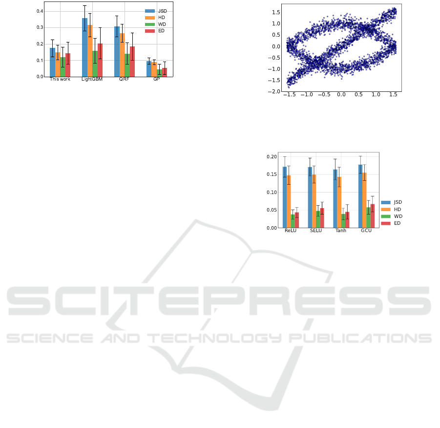
Figure 3: Average distance between the true distribution
p(y|x) and the output of each distributional predictors. The
error bars represent the mean ± one standard deviation.
We applied DN+ to this data with the hyperparame-
ters n
epoch
= 300,N
b
= 50 and b
batch
= 20 , using Tanh
layer for the activation function. All parameters of the
linear layers were initialized with random variables
drawn from N

0,0.1
2

. The obtained distributional
forecast (figure 1, right) captures aleatoric uncertainty
of the data reasonably well. The color in the figure
represents 0.5 − |Q − 0.5| , where Q ∈ [0,1] denotes
the quantile of the predictive density.
To quantitatively assess the result, we took 200
equidistant points over the interval [−1,1] of the x -axis
and, for each x in this set, sampled 3000 points from
the ensemble prediction of DN+ . Then we computed
the discrepancy between the obtained distribution and
the ground-truth distribution (15) and took the average
of the distance metric over all 200 points.
For comparison, we performed similar analyses
with three popular UQ methods: LightGBM with a
quantile loss (Ke et al., 2017), quantile regression
forests (QRF) (Meinshausen, 2006), and Gaussian pro-
cess regression (GP) (Rasmussen and Williams, 2006).
For QRF and GP we have used the implementation
of (Scikit-Garden, 2017) and (Pedregosa et al., 2011),
respectively. Hyperparameters of LightGBM and QRF
were tuned with Optuna (Akiba et al., 2019). We
computed 51 quantiles with LightGBM and QRF, and
therefrom constructed the conditional probability den-
sity p(y|x) approximately. The result was so spiky that
we had to smooth it with a Gaussian filter.
The benchmark result is summarized in figure 3.
(For the definition of four distance metrics, we re-
fer to section 5.1.) The result clearly shows that
DN+ yields better distributional forecasts than Light-
GBM and QRF. However, DN+ is outperformed by GP,
which does not come as a surprise because the ground-
truth distribution (15) is Gaussian. We once again
emphasize that the result for DN+ has been obtained
in a fully nonparametric manner without assuming any
parametric distribution such as Gaussian.
Figure 4: Average distance between the predictive distribu-
tion and the true distribution after training with four kinds
of activation functions. The error bars are one standard
deviation above and below the mean.
Figure 5: Data comprising 3000 points generated by adding
a Gaussian noise to three crossing curves.
5.4 Test on a Multimodal Synthetic
Dataset
Next, we test the proposed method on a multimodal
synthetic dataset. The data were generated from the
distributions over −π/2 ≤ x ≤ π/2,





y = x + ε,
y = cos x + ε
0
,
y = −cos x + ε
00
,
ε,ε
0
,ε
00
∼ N (0,0.15
2
). (17)
The scatter plot of the data is shown in figure 5. The
dataset includes 3000 points in total, 1000 for each
distribution. As a function of x , y is multimodal and in
general there are three peaks in the conditional proba-
bility density p(y|x).
To test the effectiveness of DN+ , we trained a NN
with the hyperparameters n
epoch
= 300 , N
b
= 50 and
b
batch
= 150 . We conducted training with four distinct
activation functions: Rectified Linear Unit (ReLU),
Scaled Exponential Linear Unit (SELU) (Klambauer
et al., 2017), Tanh activation, and Growing Cosine
Unit (GCU) (Noel et al., 2021). To measure the perfor-
mance, we took 100 equidistant points x ∈ [−π/2,π/2]
and, for each of them, computed the estimate p(
b
y|x)
via M = 10
4
ensemble prediction. The distance be-
tween p(
b
y|x) and the true conditional p(y|x) was mea-
sured with the metrics in section 5.1 and was then
averaged over all 100 points. The result is shown in
figure 5. It is observed that the scores of all four acti-
vation functions are similar, although Tanh activation
Sample-based Uncertainty Quantification with a Single Deterministic Neural Network
297

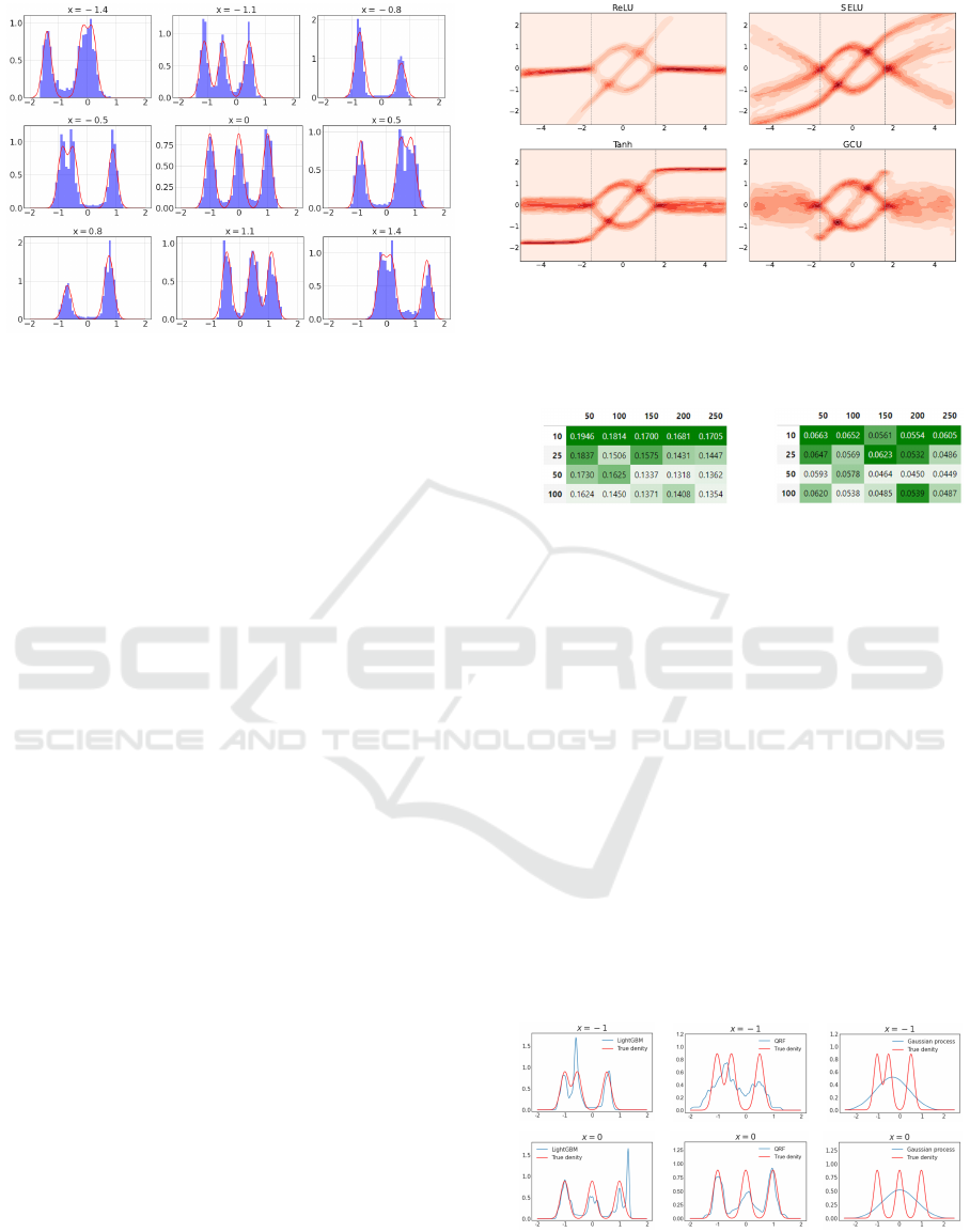
Figure 6: The histogram of the predicted conditional dis-
tribution p(
b
y|x) (blue) overlayed with the true distribution
p(y|x) (red) for the dataset in figure 5. Tanh activation was
used.
seems to perform slightly better than the others and
GCU slightly worse than the others.
To gain more insights into the approximation qual-
ity of our method, we show the predicted distribution
versus the ground truth for various values of x in fig-
ure 6. Clearly the predicted distribution reproduces
the complex multimodal shape of the true distribution
in a satisfactory manner. This is not possible with
conventional methods such as the Gaussian processes.
We have also applied plain vanilla DISCO Nets
(with no embedding layer of a random noise) to this
dataset, but it only yielded seriously corrupted esti-
mates of the predictive distribution. Actually it was
this failure that forced us to seriously consider modifi-
cations to DISCO Nets.
While all activation functions give comparable ac-
curacy of approximation for the range of data −π/2 ≤
x ≤ π/2 , what happens outside this range? Do they
still maintain similar functional forms? We have nu-
merically studied this and found, as shown in figure
7, that the four neural networks give drastically dif-
ferent extrapolations. Since no data is available for
|x| > π/2 , the epistemic uncertainty must be high and
a predictive distribution of y should have a broad sup-
port. This seems to hold true only for the network with
GCU activation. We therefore conclude that, while
the choice of an activation function hardly affects the
network’s capability to model aleatoric uncertainty for
in-distribution data, it does affect the ability to model
epistemic uncertainty for out-of-distribution data and
hence great care must be taken.
To check the hyperparameter dependence of re-
sults, we have repeated numerical experiments with
the same dataset for various sets of b
batch
and N
b
, us-
ing ReLU activation. The number of epochs n
epoch
Figure 7: Density plots of the predictive distributions for
−5 ≤ x ≤ 5 with four activation functions. Two vertical
dashed lines at x = ±π/2 indicate the boundary of the train-
ing dataset.
(a) (b)
Batchsize Batchsize
𝑁

𝑁

Figure 8: (a) Hellinger distance and (b) Wasserstein distance
between the true distribution p(y|x) and the predictive distri-
bution
b
p(y|x) computed using ReLU activation for varying
b
batch
and N
b
.
was fixed to 2 × b
batch
to keep the number of gradi-
ent updates the same across experiments, ensuring a
fair comparison. The result is shown in figure 8. It
is observed that larger N
b
and/or larger b
batch
gener-
ally leads to better (lower) scores. Note, however, that
larger N
b
entails higher numerical cost and longer com-
putational time. It is therefore advisable to make these
parameters large enough within the limit of available
computational resources, although it is likely that the
best hyperparameter values will in general depend on
the characteristics of individual datasets under consid-
eration.
In order to benchmark DN+ , we again compared
it with LightGBM, QRF and GP. We have used ReLU
activation for DN+ . Some examples of the posterior
(a) (b) (c)
Figure 9: The true density p(y|x) (red curve) and the esti-
mated density
b
p(y|x) (blue curve) obtained at x = −1 and
0 for the dataset in figure 5 using the three methods: (a)
LightGBM with quantile losses, (b) QRF, and (c) GP.
NCTA 2022 - 14th International Conference on Neural Computation Theory and Applications
298

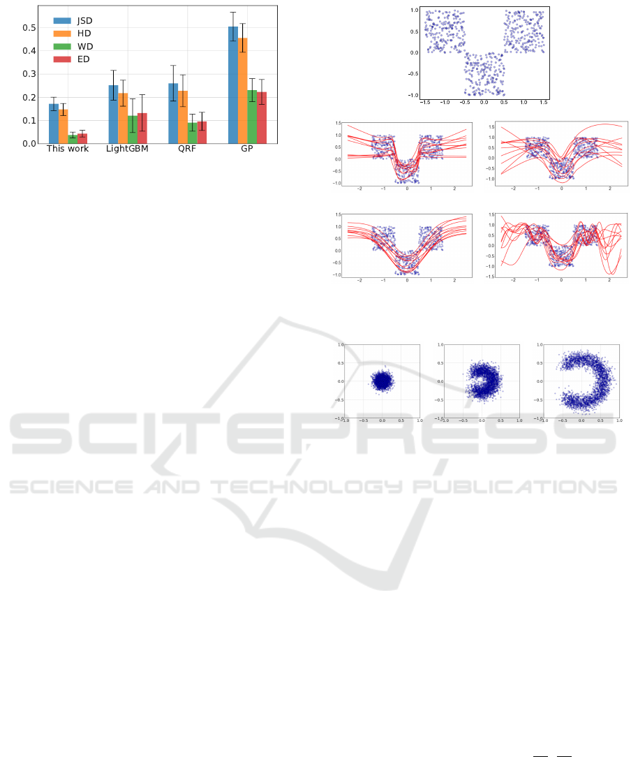
Figure 10: Comparison of DN+ against three popular UQ
methods (lower scores are better). Error bars represent the
mean ± one standard deviation.
distributions obtained with each method are displayed
in figure 9. While LightGBM and QRF seem to capture
qualitative features of the posterior well, GP entirely
misses local structures due to its inherent Gaussian
nature of the approximation.
For a quantitative comparison of the methods, we
computed the discrepancy between the estimated dis-
tribution and the true distribution and took the average
over −π/2 ≤ x ≤ π/2 . The result is displayed in fig-
ure 10. Not surprisingly, GP marked the worst score.
DN+ attained the lowest score in all the four metrics,
thus underlining the effectiveness of this approach for
modeling complex multimodal density distributions.
5.5 Sampling of Functions after Fitting
to Data
Drawing samples from a posterior predictive distribu-
tion is central to Bayesian inference (Bishop, 2006).
In GP the cost of naive generation of samples scales
cubically with the number of observations, and histor-
ically a variety of approximation schemes have been
proposed (Lázaro-Gredilla et al., 2010; Wilson et al.,
2020). In DISCO Nets and DN+ , it is in fact trivial
to sample functions from the posterior after training
on a dataset. While we make an ensemble forecast at
given x by running a forward pass with a large number
of distinct inputs a ∼ P
b
sampled from the base space
X
b
, sample functions can be obtained by simply fixing
a ∼ P
b
and running a forward pass with varying x . For
illustration, we generated a test dataset as shown in
the top panel of figure 11. In total 600 points were
generated uniformly inside three squares of size 1. We
have applied DN+ to this data with hyperparameters
n
epoch
= 50 , N
b
= 20 and b
batch
= 80 using four acti-
vation functions. For each of them we sampled 10
functions, as shown in the bottom panel of figure 11.
They cover the range of data in a similar way but per-
form qualitatively different extrapolations outside the
range of data. These characteristics that are specific
ReLU SELU
Tan h GCU
Figure 11: Data distribution (top) and samples drawn from
the fitted NN (bottom) for the four activation functions.
𝑥0 𝑥0.5 𝑥1
Figure 12: The dataset generated for the experiment with 2D
output y = (y
1
,y
2
).
to activation functions, akin to the choice of kernel
functions in GP, must be taken into consideration care-
fully when using this sampling technique for practical
purposes.
5.6 Two-dimensional Prediction
Next, we proceed to considering the case where the
response variable y is two-dimensional. As described
in section 5.2, we sample a two-dimensional random
vector a ∈ [0,1]
2
to make ensemble predictions. As a
testbed of the proposed method, we generated a dataset
from the distribution below.
y =

y
1
(x)
y
2
(x)

,
(
y
1
(x) = 0.6 cos θ × x + ε
y
2
(x) = 0.6 sin θ × x + ε
0
(18)
ε,ε
0
∼ N

0,0.1
2

, θ ∼ U

−
3π
4
,
3π
4

(19)
for 0 ≤ x ≤ 1 . The scatter plots of the data at three
values of x are displayed in figure 12. For small x ,
the data distribution is essentially isotropic, while for
larger x a gap on the left gradually opens up. The
task for DN+ is to learn this nontrivial evolution of the
distribution over the entire unit interval x ∈ [0,1] . We
Sample-based Uncertainty Quantification with a Single Deterministic Neural Network
299

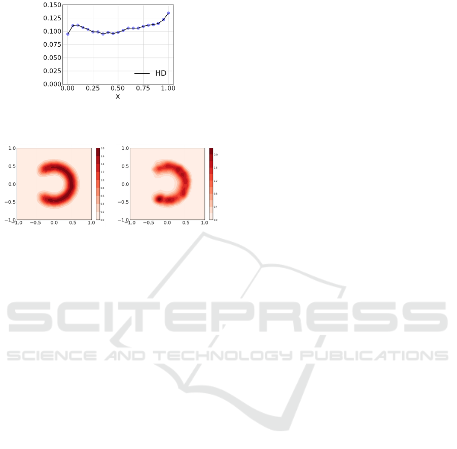
Figure 13: Density plots of the true distribution (left) and
DN+’s prediction (right) in the (y
1
,y
2
)-plane.
𝑥0.8 (truedist.) 𝑥0.8 (modeloutput)
Figure 14: Discrepancy between the true distribution p(y|x)
and the predicted distribution p(
b
y|x) measured by the
Hellinger distance based on 10
5
ensemble forecast.
have taken an equidistant grid of 3000 points over [0,1]
and generated the dataset
{
(x
i
,y
i
)
}
3000
i=1
, which was fed
to our NN. We have used ReLU activation and trained
the model with b
batch
= 300 , N
b
= 100 and n
epoch
=
300 . For various x , we made an ensemble forecast with
M = 10
5
and computed its Hellinger distance from the
true distribution (18) . The result is shown in figure 14.
The worst score was 0.135 at x = 1 and the mean over
all x was 0.106 , hence we conclude that the model
has correctly reproduced the data distribution for all
x . For illustration, we show the true distribution and
the learned distribution on the y -plane at x = 0.8 in
figure 14. Clearly, major features of the distribution are
reproduced to a good accuracy. We anticipate that the
result would be improved if the model’s layer width
is increased further and the hyperparameters of the
training such as b
batch
are optimized.
5.7 Test on Real-World Datasets
Finally we compare the performance of various base-
lines with DN+ on 10 publicly available tabular
datasets for regression tasks. For details of datasets
we refer to Appendix B. This time we have in-
cluded NGBoost (Duan et al., 2020) in the baselines,
which fits parametric distributions to data via gradi-
ent boosting of decision trees. For each dataset, we
have used 90% of the data for training and 10% for
testing. Hyperparameters of the baselines are pro-
vided in Appendix B. In DN+ , we used the hyperpa-
rameters (n
epoch
,b
batch
,N
b
) = (150,200,100) for all
datasets except for the Concrete dataset for which
(n
epoch
,b
batch
,N
b
) = (200,50,50) . In the inference
mode, M = 500 ensemble predictions were made.
QuantileTransformer(output_distribution=
’normal’) from Scikit-Learn was used to preprosess
both the input and output of the NN.
The result on the point forecast performance mea-
sured by MAE and RMSE is displayed in table 1. Over-
all, LightGBM was the best performing model and
DN+ was close to worst, although DN+ was best on
the Kin8nm dataset. This is partly as expected, since
our NN of DN+ is not optimized for achieving the
best point forecast. As is widely recognized, highly
tuned gradient boosting models often outperform plain
vanilla MLP, though we stress that DN+ can integrate
with more complex and deeper NN as well. We leave
engineering efforts for achieving better point forecast
accuracy to future work.
The probabilistic forecast performance is com-
pared in table 2. As a metric we used negative log-
likelihood (NLL) and CRPS. In order to compute NLL
numerically, we have used Gaussian KDE for the four
methods other than NGBoost. This time, DN+ was
best on average on NLL, while LightGBM was best
on average on CRPS, respectively. It should be noted
that DN+ was best on three datasets for NLL. Overall,
the probabilistic forecast performance of DN+ was at
least quite competitive with the standard baselines of
probabilistic regression. The fact that DN+ did not
clearly outperform the baselines may be indicating
that the probability distributions of the response vari-
ables in these datasets may have a simple unimodal
structure that hardly requires nonparametric methods
for complex multimodal distributions.
6 CONCLUSION
In this paper, we introduced a method DN+ built on
top of DISCO Net (Bouchacourt et al., 2016) for un-
certainty quantification with neural networks for re-
gression tasks. DN+ is a nonparametric method that
can model arbitrary complex multimodal distributions.
In contrast to Bayesian neural networks and Gaussian
processes, DN+ scales well to a large dataset without
a computational bottleneck. It also offers an easy way
to sample as many functions as desired from the pos-
terior distribution. Due to its simplicity, DN+ can be
combined with a variety of complex neural networks,
including convolutional and recurrent neural networks.
In numerical experiments, we have shown that DN+
can even model a two-dimensional distribution of a
response variable successfully, in stark contrast to con-
ventional quantile-based approaches that struggle in
NCTA 2022 - 14th International Conference on Neural Computation Theory and Applications
300

Table 1: Point forecast performance of each method on each dataset. Best result is in bold face. The lower score is better.
Dataset
MAE (↓) RMSE (↓)
QRF LGBM NGB GP
This
work
QRF LGBM NGB GP
This
work
California 0.345 0.328 0.319 0.368 0.328 0.522 0.474 0.465 0.545 0.517
Concrete 2.63 2.60 2.69 2.68 2.71 3.47 3.35 3.49 3.61 3.65
Kin8nm 0.116 0.099 0.116 0.060 0.061 0.143 0.124 0.150 0.080 0.079
Power Plant 2.37 2.30 2.37 2.60 2.73 3.40 3.22 3.39 3.63 3.76
House Sales 68.2k 63.6k 68.3k 86.0k 79.7k 123k 111k 117k 153k 166k
Elevators 1.87E-3 1.62E-3 1.58E-3 1.55E-3 1.61E-3 2.76E-3 2.36E-3 2.15E-3 2.09E-3 2.24E-3
Bank8FM 0.0227 0.0221 0.0227 0.0231 0.0223 0.0311 0.0303 0.0301 0.0307 0.0310
Sulfur 0.0172 0.0194 0.0224 0.0183 0.0197 0.0308 0.0348 0.0386 0.0302 0.0338
Superconduct 5.06 6.45 6.66 5.35 5.53 8.96 10.6 10.5 9.22 9.75
Ailerons 2.07E-4 1.07E-4 2.09E-4 1.15E-4 1.30E-4 2.64E-4 1.52E-4 2.73E-4 1.58E-4 1.84E-4
Average
Rank (↓)
2.7 2.1 3.4 2.7 3.2 3.3 2.4 3.0 2.8 3.5
Table 2: Probabilistic forecast performance of each method on each dataset. Best result is in bold face. The lower score is
better.
Dataset
NLL (↓) CRPS (↓)
QRF LGBM NGB GP
This
work
QRF LGBM NGB GP
This
work
California 0.316 0.194 0.111 0.411 0.097 0.143 0.130 0.139 0.167 0.134
Concrete 2.74 2.44 2.39 2.48 2.36 1.80 1.03 1.39 1.33 1.38
Kin8nm −0.590 −0.972 −0.869 −1.35 −0.964 0.065 0.048 0.058 0.031 0.036
Power Plant 2.27 2.16 2.11 2.39 2.33 1.16 1.04 1.14 1.24 1.27
House Sales 12.2 12.3 12.3 12.4 12.4 28.8k 26.0k 28.2k 35.9k 28.2k
Elevators −4.89 −5.09 −5.14 −5.04 −5.11 8.76E-4 7.56E-4 7.80E-4 7.65E-4 8.09E-4
Bank8FM −2.19 −2.29 −2.45 −2.39 −2.36 0.0128 0.0110 0.0105 0.0106 0.0107
Sulfur −2.89 −2.79 −2.59 −2.52 −2.72 6.30E-3 7.55E-3 9.63E-3 8.90E-3 7.79E-3
Superconduct 2.72 3.09 3.14 3.32 2.87 1.63 2.16 2.67 2.76 1.87
Ailerons −7.03 −7.72 −7.06 −7.65 −7.95 9.42E-5 5.17E-5 1.21E-4 5.55E-5 6.54E-5
Average
Rank (↓)
3.5 2.6 2.5 3.7 2.3 3.6 1.8 3.3 3.1 2.9
higher than one dimensions.
In future work, it would be interesting to apply
DN+ to uncertainty quantification problems where
images or time-series data are given as inputs to the
model.
REFERENCES
Abdar, M., Pourpanah, F., Hussain, S., Rezazadegan, D., Liu,
L., Ghavamzadeh, M., Fieguth, P., Cao, X., Khosravi,
A., Acharya, U. R., Makarenkov, V., and Nahavandi,
S. (2021). A review of uncertainty quantification in
deep learning: Techniques, applications and challenges.
Information Fusion, 76:243–297. arXiv:2011.06225.
Akiba, T., Sano, S., Yanase, T., Ohta, T., and Koyama, M.
(2019). Optuna: A Next-generation Hyperparameter
Optimization Framework. KDD ’19: Proceedings of
the 25th ACM SIGKDD International Conference on
Knowledge Discovery & Data Mining, pages 2623–
2631. arXiv:1907.10902.
Antoran, J., Allingham, J., and Hernández-Lobato, J. M.
(2020). Depth Uncertainty in Neural Networks. In
Advances in Neural Information Processing Systems
33 (NeurIPS 2020). arXiv:2006.08437.
Arpogaus, M., Voss, M., Sick, B., Nigge-Uricher, M., and
Dürr, O. (2022). Short-Term Density Forecasting of
Low-Voltage Load using Bernstein-Polynomial Nor-
malizing Flows. arXiv:2204.13939.
Bishop, C. M. (1994). Mixture density networks. Technical
Report. Aston University, Birmingham.
Bishop, C. M. (2006). Pattern Recognition and Machine
Learning. Springer.
Bouchacourt, D., Mudigonda, P. K., and Nowozin, S. (2016).
DISCO Nets : DISsimilarity COefficients Networks.
In Advances in Neural Information Processing Systems
29 (NIPS 2016). arXiv:1606.02556.
Brophy, J. and Lowd, D. (2022). Instance-Based Uncer-
tainty Estimation for Gradient-Boosted Regression
Trees. arXiv:2205.11412.
Cannon, A. J. (2011). Quantile regression neural networks:
Implementation in R and application to precipitation
downscaling. Computers & Geosciences, 37:1277–
1284.
Charpentier, B., Zügner, D., and Günnemann, S. (2020).
Posterior Network: Uncertainty Estimation without
Sample-based Uncertainty Quantification with a Single Deterministic Neural Network
301

OOD Samples via Density-Based Pseudo-Counts.
arXiv:2006.09239.
Cramer, E., Witthaut, D., Mitsos, A., and Dahmen, M.
(2022). Multivariate Probabilistic Forecasting of In-
traday Electricity Prices using Normalizing Flows.
arXiv:2205.13826.
Dabney, W., Ostrovski, G., Silver, D., and Munos, R. (2018a).
Implicit Quantile Networks for Distributional Rein-
forcement Learning. Proceedings of the 35 th Inter-
national Conference on Machine Learning, Stockholm,
Sweden, PMLR 80. arXiv:1806.06923.
Dabney, W., Rowland, M., Bellemare, M. G., and Munos,
R. (2018b). Distributional Reinforcement Learn-
ing with Quantile Regression. The Thirty-Second
AAAI Conferenceon Artificial Intelligence (AAAI-18).
arXiv:1710.10044.
Duan, T., Anand, A., Ding, D. Y., Thai, K. K., Basu, S., Ng,
A., and Schuler, A. (2020). Ngboost: Natural gradient
boosting for probabilistic prediction. Proceedings of
the 37th International Conference on Machine Learn-
ing, PMLR, pages 2690–2700. arXiv:1910.03225.
Dumas, J., Lanaspeze, A. W. D., Cornélusse, B., and Sutera,
A. (2021). A deep generative model for probabilis-
tic energy forecasting in power systems: normalizing
flows. arXiv:2106.09370.
Endres, D. M. and Schindelin, J. E. (2003). A New Metric
for Probability Distributions. IEEE Trans. Inf. Theory,
49:1858–1860.
Gal, Y. and Ghahramani, Z. (2016). Dropout as a Bayesian
Approximation: Representing Model Uncertainty in
Deep Learning. Proceedings of The 33rd International
Conference on Machine Learning, PMLR, 48:1050–
1059. arXiv:1506.02142.
Gawlikowski, J., Tassi, C. R. N., Ali, M., Lee, J., Humt, M.,
Feng, J., Kruspe, A., Triebel, R., Jung, P., Roscher, R.,
Shahzad, M., Yang, W., Bamler, R., and Zhu, X. X.
(2021). A Survey of Uncertainty in Deep Neural Net-
works. arXiv:2107.03342.
Gneiting, T. and Raftery, A. E. (2007). Strictly Proper Scor-
ing Rules, Prediction, and Estimation. Journal of the
American Statistical Association, 102:359–378.
Gneiting, T., Stanberry, L. I., Grimit, E. P., Held, L., and
Johnson, N. A. (2008). Assessing probabilistic fore-
casts of multivariate quantities, with an application to
ensemble predictionsof surface winds. Test, 17:211–
235.
Gretton, A., Borgwardt, K. M., Rasch, M. J., Schölkopf, B.,
and Smola, A. (2012). A Kernel Two-Sample Test.
Journal of Machine Learning Research, 13:723–773.
Harakeh, A. and Waslander, S. L. (2021). Estimating and
Evaluating Regression Predictive Uncertainty in Deep
Object Detectors. In ICLR 2021. arXiv:2101.05036.
Huang, G., Li, Y., Pleiss, G., Liu, Z., Hopcroft, J. E.,
and Weinberger, K. Q. (2017). Snapshot Ensem-
bles: Train 1, Get M for Free. In 5th International
Conference on Learning Representations, ICLR 2017.
arXiv:1704.00109.
Huang, G., Sun, Y., Liu, Z., Sedra, D., and Weinberger,
K. Q. (2016). Deep Networks with Stochastic Depth.
In Leibe, B., Matas, J., Sebe, N., and Welling, M.,
editors, ECCV 2016, volume 9908 of Lecture Notes in
Computer Science. arXiv:1603.09382.
Hüllermeier, E. and Waegeman, W. (2021). Aleatoric and
epistemic uncertainty in machine learning: an intro-
duction to concepts and methods. Machine Learning,
110:457–506. arXiv:1910.09457.
Jamgochian, A., Wu, D., Menda, K., Jung, S., and Kochen-
derfer, M. J. (2022). Conditional Approximate Nor-
malizing Flows for Joint Multi-Step Probabilistic
Forecasting with Application to Electricity Demand.
arXiv:2201.02753.
Ke, G., Meng, Q., Finley, T., Wang, T., Chen, W., Ma, W.,
Ye, Q., and Liu, T.-Y. (2017). LightGBM: A Highly
Efficient Gradient Boosting Decision Tree. Advances
in Neural Information Processing Systems 30 (NIPS
2017), pages 3149–3157.
Klambauer, G., Unterthiner, T., Mayr, A., and Hochreiter,
S. (2017). Self-Normalizing Neural Networks. 31st
Conference on Neural Information Processing Systems
(NIPS 2017). arXiv:1706.02515.
Kobyzev, I., Prince, S. J., and Brubaker, M. A. (2021).
Normalizing Flows: An Introduction and Review of
Current Methods. IEEE Transactions on Pattern
Analysis and Machine Intelligence, 43(11):3964–3979.
arXiv:1908.09257.
Kullback, S. and Leibler, R. (1951). On information and
sufficiency. Annals of Mathematical Statistics, 22:79–
86.
Lahlou, S., Jain, M., Nekoei, H., Butoi, V., Bertin, P.,
Rector-Brooks, J., Korablyov, M., and Bengio, Y.
(2021). DEUP: Direct Epistemic Uncertainty Predic-
tion. arXiv:2102.08501.
Lakshminarayanan, B., Pritzel, A., and Blundell, C. (2017).
Simple and Scalable Predictive Uncertainty Estima-
tion using Deep Ensembles. Advances in Neu-
ral Information Processing Systems 30 (NIPS 2017).
arXiv:1612.01474.
Lampinen, J. and Vehtari, A. (2001). Bayesian approach
for neural networks—review and case studies. Neural
Networks, 14:257–274.
Lázaro-Gredilla, M., Quiñonero-Candela, J., Rasmussen,
C. E., and Figueiras-Vidal, A. R. (2010). Sparse Spec-
trum Gaussian Process Regression. Journal of Machine
Learning Research, 11:1865–1881.
Ma, X., Xia, L., Zhou, Z., Yang, J., and Zhao, Q. (2020).
DSAC: Distributional Soft Actor Critic for Risk-
Sensitive Reinforcement Learning. arXiv:2004.14547.
Maddox, W. J., Izmailov, P., Garipov, T., Vetrov, D. P., and
Wilson, A. G. (2019). A Simple Baseline for Bayesian
Uncertainty in Deep Learning. In Advances in Neural
Information Processing Systems 32 (NeurIPS 2019).
arXiv:1902.02476.
Meinshausen, N. (2006). Quantile Regression Forests. Jour-
nal of Machine Learning Research, 7:983–999.
März, A. and Kneib, T. (2022). Distributional Gradient
Boosting Machines. arXiv:2204.00778.
Nguyen-Tang, T., Gupta, S., and Venkatesh, S. (2021). Distri-
butional Reinforcement Learning via Moment Match-
ing. The Thirty-Fifth AAAI Conference on Artificial
Intelligence (AAAI-21). arXiv:2007.12354.
NCTA 2022 - 14th International Conference on Neural Computation Theory and Applications
302

Nikulin, M. S. (2001). Hellinger distance. Encyclopedia of
Mathematics, EMS Press.
Noel, M. M., L , A., Trivedi, A., and Dutta, P. (2021). Grow-
ing Cosine Unit: A Novel Oscillatory Activation Func-
tion That Can Speedup Training and Reduce Parame-
ters in Convolutional Neural Networks.
Pacchiardi, L., Adewoyin, R., Dueben, P., and Dutta,
R. (2021). Probabilistic Forecasting with Gen-
erative Networks via Scoring Rule Minimization.
arXiv:2112.08217.
Papamakarios, G., Nalisnick, E., Rezende, D. J., Mo-
hamed, S., and Lakshminarayanan, B. (2021). Nor-
malizing Flows for Probabilistic Modeling and Infer-
ence. Journal of Machine Learning Research, 22:1–64.
arXiv:1912.02762.
Pearce, T., Leibfried, F., and Brintrup, A. (2020). Uncer-
tainty in Neural Networks: Approximately Bayesian
Ensembling. Proceedings of the Twenty Third Interna-
tional Conference on Artificial Intelligence and Statis-
tics, PMLR, 108:234–244. arXiv:1810.05546.
Pedregosa, F., Varoquaux, G., Gramfort, A., Michel, V.,
Thirion, B., Grisel, O., Blondel, M., Prettenhofer, P.,
Weiss, R., Dubourg, V., Vanderplas, J., Passos, A.,
Cournapeau, D., Brucher, M., Perrot, M., and Duch-
esnay, E. (2011). Scikit-learn: Machine Learning
in Python. Journal of Machine Learning Research,
12:2825–2830.
Pinson, P. and Girard, R. (2012). Evaluating the quality of
scenarios of short-term wind power generation. Ap-
plied Energy, 96:12–20.
Rasmussen, C. E. and Williams, C. K. I. (2006). Gaussian
Processes for Machine Learning. MIT Press.
Rittler, N., Graziani, C., Wang, J., and Kotamarthi, R. (2022).
A Deep Learning Approach to Probabilistic Forecast-
ing of Weather. arXiv:2203.12529.
Scikit-Garden (2017). https://github.com/scikit-garden/
scikit-garden.
Sejdinovic, D., Sriperumbudur, B., Gretton, A., and Fuku-
mizu, K. (2013). Equivalence of distance-based and
RKHS-based statistics in hypothesis testing. Ann.
Statist., 41:2263–2291. arXiv:1207.6076.
Sendera, M., Tabor, J., Nowak, A., Bedychaj, A., Patacchi-
ola, M., Trzcinski, T., Spurek, P., and Zieba, M. (2021).
Non-Gaussian Gaussian Processes for Few-Shot Re-
gression. Advances in Neural Information Processing
Systems 34 (NeurIPS 2021). arXiv:2110.13561.
Shen, C. and Vogelstein, J. T. (2018). The Exact Equiva-
lence of Distance and Kernel Methods for Hypothesis
Testing. arXiv:1806.05514.
Sick, B., Hothorn, T., and Dürr, O. (2020). Deep trans-
formation models: Tackling complex regression prob-
lems with neural network based transformation models.
arXiv:2004.00464.
Singh, R., Lee, K., and Chen, Y. (2022). Sample-based Dis-
tributional Policy Gradient. Proceedings of The 4th
Annual Learning for Dynamics and Control Confer-
ence, PMLR, 168:676–688. arXiv:2001.02652.
Sprangers, O., Schelter, S., and de Rijke, M. (2021). Prob-
abilistic gradient boosting machines for large-scale
probabilistic regression. Proceedings of the 27th ACM
SIGKDD Conference on Knowledge Discovery & Data
Mining. arXiv:2106.01682.
Szekely, G. J. (2003). E-statistics: Energy of Statistical
Samples. Bowling Green State University, Department
of Mathematics and Statistics Technical Report No.
03–05.
Szekely, G. J. and Rizzo, M. L. (2004). Testing for Equal
Distributions in High Dimension. InterStat. November
(5).
Szekely, G. J. and Rizzo, M. L. (2013). Energy statistics:
A class of statistics based on distances. Journal of
Statistical Planning and Inference, 143:1249–1272.
Szekely, G. J. and Rizzo, M. L. (2017). The Energy of
Data. Annual Review of Statistics and Its Application,
4:447–479.
Tagasovska, N. and Lopez-Paz, D. (2019). Single-
Model Uncertainties for Deep Learning. In Proceed-
ings of the 33rd International Conference on Neu-
ral Information Processing Systems (NeurIPS 2019).
arXiv:1811.00908.
Wilson, J., Borovitskiy, V., Terenin, A., Mostowsky, P., and
Deisenroth, M. (2020). Efficiently sampling functions
from Gaussian process posteriors. Proceedings of the
37th International Conference on Machine Learning,
PMLR, 119:10292–10302. arXiv:2002.09309.
Yang, D., Zhao, L., Lin, Z., Qin, T., Bian, J., and Liu, T.
(2019). Fully Parameterized Quantile Function for Dis-
tributional Reinforcement Learning. 33rd Conference
on Neural Information Processing Systems (NeurIPS
2019). arXiv:1911.02140.
Zhang, P., Chen, X., Zhao, L., Xiong, W., Qin, T., and
Liu, T.-Y. (2021). Distributional Reinforcement Learn-
ing for Multi-Dimensional Reward Functions. 35th
Conference on Neural Information Processing Systems
(NeurIPS 2021). arXiv:2110.13578.
APPENDIX
A Minimizer of the Loss Function
As mentioned in section 3, the energy score (7) is a strictly
proper scoring rule, making it an ideal tool for distributional
learning. However, the underlying mathematics (Szekely,
2003) may not be easily accessible for practitioners of data
science. In this appendix, we present a short and rudimen-
tary argument highlighting that NN training based on the
energy score does indeed allow to learn the correct predictive
distribution.
Let us begin by observing that, when the loss (8) is
averaged over all data in the minibatch, it approximately
holds that
1
b
batch
b
batch
∑
k=1
L

y
k
,

b
y
(n)
k

N
b
n=1

'
Z
dx p(x)

Z
dy p(y|x)
Z
d
b
y p(
b
y|x)ky −
b
yk
−
1
2
Z
d
b
y p(
b
y|x)
Z
d
b
y
0
p(
b
y
0
|x)k
b
y −
b
y
0
k

(20)
Sample-based Uncertainty Quantification with a Single Deterministic Neural Network
303

where p(y|x) is the true conditional distribution and p(
b
y|x)
is the predicted distribution by the model. To stress that
they are different functions, we will hereafter write p(y|x)
as p
x
(y) and p(
b
y|x) as f
x
(y) , respectively. Our interest is in
the stationary point(s) of the loss function as a functional of
f
x
(y) . Before taking the functional derivative w.r.t. f
x
, we
must take note of the fact that
R
dy f
x
(y) = 1 . Introducing
a Lagrangian multiplier function λ(x) , we obtain the loss
functional
Z
dx p(x)
Z
dy
Z
dy
0

p
x
(y) f
x
(y
0
) −
1
2
f
x
(y) f
x
(y
0
)

× ky − y
0
k −
Z
dx λ(x)

Z
dy f
x
(y) − 1

. (21)
Differentiation w.r.t. f
x
(y) yields the saddle point equation
Z
dy
0

p
x
(y
0
) − f
x
(y
0
)

ky − y
0
k =
λ(x)
p(x)
. (22)
Let us consider the case where y is a scalar. Using
∂
2
y
|y − y
0
| = 2δ(y − y
0
) we may take the second derivative
of both sides of (22) and obtain f
x
(y) = p
x
(y) . This means
that the model’s prediction agrees with the true conditional
distribution, which is the desired result.
Actually this mathematical trick applies to arbitrary odd
dimensions. For illustration, suppose y is in three dimen-
sions. The radial component of the Laplacian in three dimen-
sions is given by
∆g(r) =
1
r
2
∂
r

r
2
∂
r
g(r)

(23)
for r =
q
x
2
1
+ x
2
2
+ x
2
3
, so
∆
2
r = ∆(∆r) ∝ ∆
1
r
∝ δ(x). (24)
In the last step we have used the fact that 1/r is the
Green’s function of the Poisson equation in three dimen-
sions. Therefore, acting ∆
y
on both sides of (22) yields
f
x
(y) − p
x
(y) = 0.
The case of even dimensions needs a little more caution.
Let κ(a,b) := ka − bk . Suppose g(a) =
R
db κ (a, b) f (b)
holds for some functions f and g . Then it is easy to verify
that f (c) =
R
da κ
−1
(c,a)g(a) , where the inverse of κ is
defined by the relation
Z
da κ
−1
(c,a)κ(a,b) = δ(c − b). (25)
Using this for (22) we formally obtain
p
x
(y) − f
x
(y) =
λ(x)
p(x)
Z
dy
0
κ
−1
(y,y
0
). (26)
We compute κ
−1
in the momentum space since convolution
becomes an algebraic product. Let
kak =
Z
d
d
q
(2π)
d
e
ia·q
µ(q). (27)
Then
µ(q) =
Z
db e
−iq·b
kbk (28)
= lim
ε→+0
Z
db e
−εkbk−iq·b
kbk. (29)
For d = 2, a careful calculation shows that
µ(q) = −
2π
kqk
3
. (30)
Therefore
κ
−1
(y,y
0
) = −
1
2π
Z
d
2
p
(2π)
2
e
i(y−y
0
)·p
kpk
3
(31)
=
1
2π
∆
y
0
Z
d
2
p
(2π)
2
e
i(y−y
0
)·p
kpk (32)
= −
1
4π
2
∆
y
0
1
ky − y
0
k
3
. (33)
Plugging this into (26) yields p
x
(y) = f
x
(y) , as desired.
Here we have used the fact that the integral of a total deriva-
tive vanishes due to the absence of a surface contribution.
The argument above generalizes to higher even d.
B Summary of Real-World Datasets
Below is the summary of the datasets used for the benchmark
test in section 5.7.
Dataset Size dim(x) URL
California 20640 8
https://scikit-learn.org/stable/
modules/generated/sklearn.
datasets.fetch_california_
housing.html
Concrete 1030 8
https://www.openml.org/d/4353
Kin8nm 8192 8
https://www.openml.org/d/189
Power Plant 9568 4
https://archive.ics.uci.edu/ml/
datasets/combined+cycle+
power+plant
House Sales 21613 19
https://www.openml.org/d/42635
Elevators 16599 18
https://www.openml.org/d/216
Bank8FM 8192 8
https://www.openml.org/d/572
Sulfur 10081 5
https://www.openml.org/d/23515
Superconduct 21263 81
https://www.openml.org/d/43174
Ailerons 13750 33
https://www.openml.org/d/44137
Remarks:
• The number of trees in QRF was set to 1000.
• The number of trees in LightGBM was set to 300.
learning_rate and min_child_weight were tuned.
• The number of trees in NGBoost was set to 500.
learning_rate was tuned. The Gaussian distribution
was used for fitting.
• GP’s kernel used the sum of the isotropic Matern
kernel and the white kernel. QuantileTransformer
(output_distribution=’normal’) from Scikit-
Learn was used to preprosess the input, and
RobustScaler() from Scikit-Learn was used to scale
the output.
• To calculate CRPS we have used the li-
brary properscoring available at https:
//github.com/TheClimateCorporation/properscoring.
NCTA 2022 - 14th International Conference on Neural Computation Theory and Applications
304