
Approaches for Rule Discovery in a Learning Classifier System
Michael Heider
a
, Helena Stegherr
b
, David P
¨
atzel
c
, Roman Sraj, Jonathan Wurth
d
,
Benedikt Volger and J
¨
org H
¨
ahner
e
Universit
¨
at Augsburg, Am Technologiezentrum 8, Augsburg, Germany
fi
Keywords:
Rule Set Learning, Rule-based Learning, Learning Classifier Systems, Evolutionary Machine Learning,
Interpretable Models, Explainable AI.
Abstract:
To fill the increasing demand for explanations of decisions made by automated prediction systems, machine
learning (ML) techniques that produce inherently transparent models are directly suited. Learning Classifier
Systems (LCSs), a family of rule-based learners, produce transparent models by design. However, the use-
fulness of such models, both for predictions and analyses, heavily depends on the placement and selection
of rules (combined constituting the ML task of model selection). In this paper, we investigate a variety of
techniques to efficiently place good rules within the search space based on their local prediction errors as well
as their generality. This investigation is done within a specific LCS, named SupRB, where the placement of
rules and the selection of good subsets of rules are strictly separated in contrast to other LCSs where these
tasks sometimes blend. We compare a Random Search, (1, λ)-ES and three Novelty Search variants. We find
that there is a definitive need to guide the search based on some sensible criteria, i.e. error and generality,
rather than just placing rules randomly and selecting better performing ones but also find that Novelty Search
variants do not beat the easier to understand (1,λ)-ES.
1 INTRODUCTION
With the ever increasing automation in many
socio-technical settings, such as manufacturing, au-
tonomous decisions of agents are more common than
ever. This advent of more independent and intelli-
gent technical systems holds great potentials in in-
creasing safety and comfort of workers as well as gen-
eral productivity. However, the roll-out of such sys-
tems can be held back when stakeholders, from op-
erator to management level, do not trust that the sys-
tems perform on-par or even better than their human
counterparts. Therefore, agents are required to give
those stakeholders sensible explanations and insights
into their decision making processes. (Heider et al.,
2022a)
For the machine learning components of such
agents, this means that they should offer strong inter-
pretability, self-explaining or transparency-by-design
capabilities. Recently, the use of Learning Classi-
a
https://orcid.org/0000-0003-3140-1993
b
https://orcid.org/0000-0001-7871-7309
c
https://orcid.org/0000-0002-8238-8461
d
https://orcid.org/0000-0002-5799-024X
e
https://orcid.org/0000-0003-0107-264X
fier Systems (LCSs) (Urbanowicz and Moore, 2009)
in such scenarios was proposed by (Heider et al.,
2021). They argue that LCSs are uniquely suited
as this family of rule-based learning algorithms fea-
tures both powerful machine learning capabilities in
all commonly encountered settings as well as inher-
ently transparent models that follow human thought
processes due to their rule-like structure. Rules in an
LCS are of an if-then form, where the if (or condi-
tion) constricts the section of the feature space this
rule applies to (matches) and the then contains a sim-
pler, therefore more comprehensible, local model able
to predict data points from that feature space partition.
Conditions are usually optimized using a stochastic
search heuristic, such as evolutionary algorithms. The
model’s practical transparency (or explainability in a
broader context) is primarily influenced by the num-
ber of rules present and their placement within the
feature space (the two tasks that constitute model
selection in rule-based machine learning). There-
fore, the—as optimal as possible—placement of rules
should be a primary concern when designing an LCS
algorithm with explainability requirements.
In this work, we expand the Supervised Rule-
based learning system (SupRB) (Heider et al., 2022b),
Heider, M., Stegherr, H., Pätzel, D., Sraj, R., Wurth, J., Volger, B. and Hähner, J.
Approaches for Rule Discovery in a Learning Classifier System.
DOI: 10.5220/0011542000003332
In Proceedings of the 14th International Joint Conference on Computational Intelligence (IJCCI 2022), pages 39-49
ISBN: 978-989-758-611-8; ISSN: 2184-3236
Copyright © 2023 by SCITEPRESS – Science and Technology Publications, Lda. Under CC license (CC BY-NC-ND 4.0)
39

a recently proposed LCS for regression tasks, with
different methods to discover new rules that fit the
data well and benchmark them against each other on
a variety of real world datasets.
2 LEARNING CLASSIFIER
SYSTEMS AND RULE
DISCOVERY
As previously introduced, LCSs are a family of—
typically evolutionary—rule-based learning systems
with a long research history (Urbanowicz and Moore,
2009; Urbanowicz and Browne, 2017). Traditionally,
they are categorized into two approaches:
• Michigan-style systems which feature strong on-
line learning capabilities and have evolved from
reinforcement learning (RL) to all major learning
schemes. They consist of a single population of
rules on which the optimizer operates directly.
• Pittsburgh-style systems that typically perform of-
fline batch learning and primarily focus on super-
vised learning and feature a population of sets of
rules, where the optimizer operates on those sets
rather than the rules individually.
Due to those very different outsets, their approach
to rule discovery and improvement differs substan-
tially. For example, the most widespread Michigan-
style system, the XCS classifier system (Wilson,
1995), does feature two mechanisms to determine a
new rule. The first is the covering mechanism. When
the number of rules that match a new data point falls
below a predetermined threshold, new rules are gen-
erated that match this data point. These rules are often
randomly made more general than to just match this
point specifically and therefore slightly differ when
inserted into the population of rules. The second is
the evolutionary algorithm. It is invoked on match-
ing rules that also propose the chosen action (e.g. fol-
lowing an epsilon-greedy policy in RL). It utilizes
crossover and mutation mechanisms appropriate for
the types of input data and evolves the population in a
steady-state manner.
For Pittsburgh-style systems, new rules can be di-
rectly added to an individual of the population (a set
of rules), shared between individuals or be the product
of a mutation (and more rarely rule-level crossover)
operator. As the evolutionary algorithm of these sys-
tems operates on rule sets rather than rules directly,
the fitness signal that guides evolution is not based
on individual rule performance but rather the perfor-
mance of a given set of rules, which can complicate
rule discovery due to the added indirection.
3 THE SUPERVISED
RULE-BASED LEARNING
SYSTEM
The Supervised Rule-based learning system (SupRB)
(Heider et al., 2022b) is an LCS with alternating
phases of rule discovery and solution composition
(additional details in (Heider et al., 2022c)). The two
phases combined solve the standard machine learning
task of model selection for an LCS. Splitting these
phases allows a more direct control of the optimiza-
tion process as objectives are more directly related
to overall behaviour. In contrast, in Pittsburgh-style
systems a model’s fitness that also controls changes
made to its rules follows the interaction of its rules
rather than their individual suitability, whereas, in
Michigan-style systems, rule fitness often depends on
their neighbouring rules (niching) and, due to their
online learning nature, does not necessarily relate to
the full dataset. In the rule discovery (RD) phase of
SupRB, new rules are generated and locally optimized
to produce a diverse pool of general rules that exhibit
low errors. Subsequently, in the solution composition
(SC) phase, an optimizer attempts to select a well per-
forming subset of the discovered rules. This subset
should be small (exhibiting low complexity) but also
produce a model (by mixing rules in areas of over-
lap) with a low prediction error. There is an obvi-
ous tradeoff between those two objectives (as was be-
tween general and accurate rules during RD). Thus,
balancing these objectives highly depends on the use
case at hand and the inherent requirements into expla-
nations and model readability. In some cases, larger
models might be acceptable, whereas, in others, e.g.
when decisions need to be made fast, smaller models
with less overlap are preferred.
The alternation between phases (rather than hav-
ing a very long RD phase followed by an SC phase)
allows to use additional information and guide the op-
timizers better. When discovering new rules, the RD
mechanism places new rules more likely where the
last elitist from the SC process showed high predic-
tion errors. This can allow to fill unmatched areas (or
areas of ill-fit local models) in the overall model that
might otherwise go unnoticed. Blindly fitting a mul-
titude of rules would become quite expensive as the
whole dataset needs to be matched and then batch-
learned multiple times. Additionally, it is hard to de-
termine beforehand how many rules would be needed
in the pool to find a satisfactory subset that solves the
learning task.
SupRB’s model is kept as simple and interpretable
as possible as its transparency is a central aspect (Hei-
der et al., 2022b):
ECTA 2022 - 14th International Conference on Evolutionary Computation Theory and Applications
40

1. Rules’ conditions use an interval based matching:
A rule k applies for example x iff x
i
∈ [l
k,i
,u
k,i
]∀i
with l being the lower and u the upper bounds.
2. Rules’ local models f
k
(x) are linear. They are
fit using linear least squares with a l2-norm reg-
ularization (Ridge Regression) on the subsample
matched by the respective rule.
3. When mixing multiple rules to make a predic-
tion, a rule’s experience (the number of examples
matched during training and therefore included in
fitting the submodel) and in-sample error are used
in a weighted sum.
For the SC phase optimizer, we use a genetic al-
gorithm (GA) for all experiments in this paper. It op-
erates directly on a bitmap corresponding to whether
a rule from the pool is part of this solution to the
learning task at hand or whether it is not. In previ-
ous work by (Wurth et al., 2022) other metaheuristic
optimizers were tested to compose solutions. They
found that the choice of metaheuristic is—given suf-
ficient computational budget—largely dependent on
the learning task, although even there, differences
were small, which makes the GA a fitting choice.
This is also the more traditional option as LCSs typi-
cally feature evolutionary computation methods. Par-
ent (groups of two) selection is done using tourna-
ment selection. Those parents are recombined with
an n-point crossover under a 90% probability. The
children are then mutated using a probabilistic bit-flip
mutation. These children form the new population
together with the fittest parents (elitism). In our ex-
periments we used a population size of 32 children
and 5 to 6 elitists. An individual’s (solution to the
learning task) fitness is determined based on its in-
sample prediction error and its complexity (number of
rules present) following (Heider et al., 2022b). Criti-
cally, this phase does not affect the position of rules’
bounds. Individuals can only be composed of rules
in the pool and those rules remain unchanged by the
GA’s operators.
The main subject of this paper is the RD phase’s
optimizer. In contrast to many typical optimization
problems we do not want to find the singular glob-
ally optimal rule but rather a set of localized rules that
perform well in this particular feature space partition,
thus, we are attempting to find an unknown number of
local optima without mapping the entire fitness land-
scape. The rules discovered should be a diverse set
and we can allow overlapping rules as SC will se-
lect the subset of discovered rules most appropriate
to solve the learning task. As for the SC, a variety of
different optimizers can achieve this. In the follow-
ing, the five different optimization approaches for RD
that will be compared in the remainder of this paper
are presented. For all heuristics we utilize the same
approach for calculating rule fitness by combination
of two objectives, utilizing the in-sample error and
the matched feature space volume, respectively—cf.
(Heider et al., 2022b).
3.1 Evolution Strategy
As discussed before, LCSs traditionally apply some
evolutionary algorithm for their optimization pro-
cesses. Therefore, the first strategy employed for RD
in SupRB, which was also used for the experiments
in (Wurth et al., 2022), is an Evolution Strategy (ES)
(Heider et al., 2022b), specifically, a simplified (1,λ)-
ES. The initial individual for the ES is generated by
placing a rule at a randomly selected training exam-
ple, preferring those examples where the in-sample
error is high in the intermediate global solution. This
individual serves as the initial candidate for addition
to the pool and the parent. From the parent, λ children
are generated, each mutated by a non-adaptive oper-
ator which moves the upper and lower bounds fur-
ther outwards by adding values sampled from a half-
normal distribution. The parent for the next gener-
ation is the child individual with the highest fitness.
If this individual showed a better fitness than the cur-
rent candidate it also becomes the new candidate. The
evolutionary search terminates when for a fixed num-
ber of generations no new candidate has been found.
This ES produces one rule at a time but can easily
be parallelized. One merit of this approach is in the
explainability of both the search procedure and the re-
sulting pool. In general, rules that have fitnesses inde-
pendent from other rules are easier to understand for
most non-experts. Whereas, in most current LCSs,
the fitness assigned to a rule is highly dependent on
what other rules it is surrounded by. Beyond fitness-
based considerations on the understandability of our
approach, the ES is also a quite easy to follow search
method: Expand the area (or hypervolume) an indi-
vidual matches, evaluate the new individuals, choose
the best new option and repeat.
3.2 Random Search
As an alternative to the strongly fitness-guided RD
performed by the ES, Random Search (RS) is intro-
duced. RS commonly serves as a baseline for test-
ing the performance of other optimization algorithms.
Furthermore, with the ulterior motive of finding di-
verse rules to add to the pool, RS provides an inter-
esting approach where the fitness only plays a role in
the selection of the final candidate, but not in the gen-
eration of new rules.
Approaches for Rule Discovery in a Learning Classifier System
41

In SupRB, RS, similarly to ES, randomly selects
a fixed number of data points weighted by their re-
spective in-sample prediction errors in the last solu-
tion candidate (produced by the previous SC phase).
We then place random bounds around those points
based on half-normal distributions (to ensure we al-
ways match the selected point). To balance the com-
putational cost between RD approaches, we produce
substantially more rules initially than we would in an
ES generation. We then greedily select the rule with
the highest fitness to become part of the pool.
3.3 Novelty Search
One of the central issues of RD is that the optimizer
is tasked to find multiple rules that partition the fea-
ture space and, in their individual area, predict data
points well, whereas in many typical optimization
problems the optimizer would be expected to find a
single global optimum (or at least a point very close to
it). This task the optimizer has to complete can some-
what be viewed as being tasked to map the larger local
optima within the search space. We aim at finding a
diverse set of good rules, each within their specific
area.
In this section, we describe an approach based on
Lehman’s Novelty Search (NS) (Lehman, 2012). In
this evolutionary search method the optimizer is not
(or not fully) guided by the typical fitness function
but rather tries to find individuals that exhibit new be-
haviour previously unknown within the population.
Mapped to our case, where we want to find a rule
that predicts an area of the feature space currently
unmatched or only matched by rules with high er-
rors in this area, behaviour of rules can be equated to
what subsample of the training data they match. For
our adaptation, we base the NS on a (µ , λ)-ES with
elitism and follow the extensive experimental findings
laid out by (Gomes et al., 2015). In each iteration, we
select a list of λ parents out of the current population.
These parents are paired, undergo a uniform crossover
and a half-normal mutation (cf. Section 3.1). The re-
sulting children are then fitted and the best performing
µ children are selected for the next population. Addi-
tionally, we select a number of high-performing par-
ents equal to the number of rules the NS is expected to
produce within one RD phase as part of the new pop-
ulation (elitism). Performance of an individual can be
based on novelty alone or on a combination of fitness
(as used in the ES; cf. Section 3.1) and novelty, e.g. a
linear combination. For the novelty of a rule, we com-
pare its match set and the match sets of the other rules
in the pool and the current NS population (the other
children for the selection or the parents for elitism,
respectively). The novelty score assigned to a rule is
the average Hamming-distance between its match set
and its k nearest neighbours’ (most similar rules). k is
set to 15; a value typically encountered with other NS
applications in literature—e.g. (Lehman and Stanley,
2010). After a set number of iterations, we add a set
number of rules to the pool and conclude this phase.
Which rules get added can be randomized or based on
the highest novelty(-fitness combination).
In addition to the basic NS, we implemented and
experimented with two variants: Minimal Criteria
Novelty Search (MCNS) (Lehman and Stanley, 2010;
Lehman, 2012) and Novelty Search with Local Com-
petition (NSLC) (Lehman, 2012).
MCNS imposes additional pressure on the search
to explore less vividly and focus more on rules that
at least fulfil some minimal requirement. In our ex-
periments, we set the minimal criterion to a minimum
number (tuned between 10 and 20) of examples from
the training data having to be matched by the rule to
become viable. Although, we did also impose that at
most one fourth of the population should be removed
because they missed the minimal criterion to prevent
collapsing gene pools. We also use progressive mini-
mal criteria novelty search (Gomes et al., 2012), itself
based on MCNS, as an option for combining fitness
and novelty as the objective. Here, all individuals that
do exhibit a fitness worse than the median fitness are
removed automatically in each iteration of the search.
This approach is not tied to MCNS and can be used in
all three variants.
NSLC introduces a localised fitness-based pres-
sure on the new generation. The idea is that, within
a neighbourhood (based on their behaviour and not
their position in the search space) of similar rules, the
rules that exhibit high fitnesses should be chosen. A
rule’s novelty score gets increased by a factor of b/κ,
where b is the number of individuals within the neigh-
bourhood specified by κ that have a worse fitness than
the rule currently evaluated. We chose κ to be equal
to k as this already does specify a neighbourhood of
rules this rule is in competition with.
One disadvantage of NS-like approaches is that
rule selection is no longer solely based on indepen-
dent metrics (fitness) but rather on the independent
fitness and the highly dependent (on other rules) nov-
elty score.
4 EVALUATION
To examine the differences between the rule dis-
covery methods and to find the most versatile strategy,
ECTA 2022 - 14th International Conference on Evolutionary Computation Theory and Applications
42

we evaluated those strategies within SupRB on
several regression datasets.
4.1 Experiment Design
SupRB is implemented
1
in Python 3.9, adhering to
scikit-learn (Pedregosa et al., 2011) conventions. In-
put features are transformed into the range [−1, 1],
while the target is standardized. Both transforma-
tions are reversible but improve SupRB’s training pro-
cess as they help preventing rules to be placed in re-
gions where no sample could be matched and remove
the need to tune error coefficients in fitness calcula-
tions, respectively. Based on our assumptions about
the number of rules needed, 32 cycles of alternat-
ing rule discovery and solution composition are per-
formed, generating four (or 8 in case of NS vari-
ants) rules in each cycle for a total of 128 (256 for
NS variants) rules. Additionally, the GA is con-
figured to perform 32 iterations with a population
size of 32. To tune some of the more sensitive pa-
rameters, we performed a hyperparameter search us-
ing a Tree-structured Parzen Estimator in the Optuna
framework (Akiba et al., 2019) that optimizes aver-
age solution fitness on 4-fold cross validation. We
tuned the optimizers on each dataset independently
for a fixed tuning budget of 360 core hours. The final
evaluation, for which we report results in Section 4.2,
uses 8-split Monte Carlo cross-validation, each with
25% of samples reserved as a validation set. Each
learning algorithm is evaluated with 8 different ran-
dom seeds for each 8-split cross-validation, resulting
in a total of 64 runs.
Table 1: Overview of the regression datasets the five rule
discovery approaches for SupRB are compared on.
Name n
dim
n
sample
Combined Cycle Power Plant 4 9568
Airfoil Self-Noise 5 1503
Concrete Strength 8 1030
Energy Efficiency Cooling 8 768
We evaluate on four datasets part of the UCI Ma-
chine Learning Repository (Dua and Graff, 2017).
An overview of sample size and dimensionality is
given in Table 1. The Combined Cycle Power Plant
(CCPP) (Kaya and T
¨
ufekci, 2012; T
¨
ufekci, 2014)
dataset shows an almost linear relation between fea-
tures and targets and can be acceptably accurately
predicted using a single rule. Airfoil Self-Noise
1
Recent code at: https://github.com/heidmic/suprb. The
specific version of the code used in this paper can be found
at: https://doi.org/10.5281/zenodo.7059913.
(ASN) (Brooks et al., 1989) and Concrete Strength
(CS) (Yeh, 1998) are both highly non-linear and will
likely need more rules to predict the target suffi-
ciently. The CS dataset has more input features than
ASN but is easier to predict overall. Energy Effi-
ciency Cooling (EEC) (Tsanas and Xifara, 2012) is
another rather linear dataset, but has a much higher
input features to samples ratio compared to CCPP. It
should similarly be possible to model it using only
few rules.
4.2 Results
In the following we abbreviate SupRB using X as RD
method simply by X.
The means and standard deviations of model per-
formances (measured using the—standardized indi-
vidually per dataset—mean squared error on test data
(MSE)) and model complexities (measured by the
number of rules in the final elitist) achieved by the
five RD approaches when evaluated—as described in
the previous section—on the four real-world datasets
are given in Tables 2 and 3. At first glance, on all four
datasets, RS shows the worst performance in terms of
mean MSE and, with the exception of CS, the mod-
els it creates also have the highest model complexity.
The other four optimization approaches vary in their
results between datasets.
In order to get a better overview as well as include
distributional information, we create violin plots to
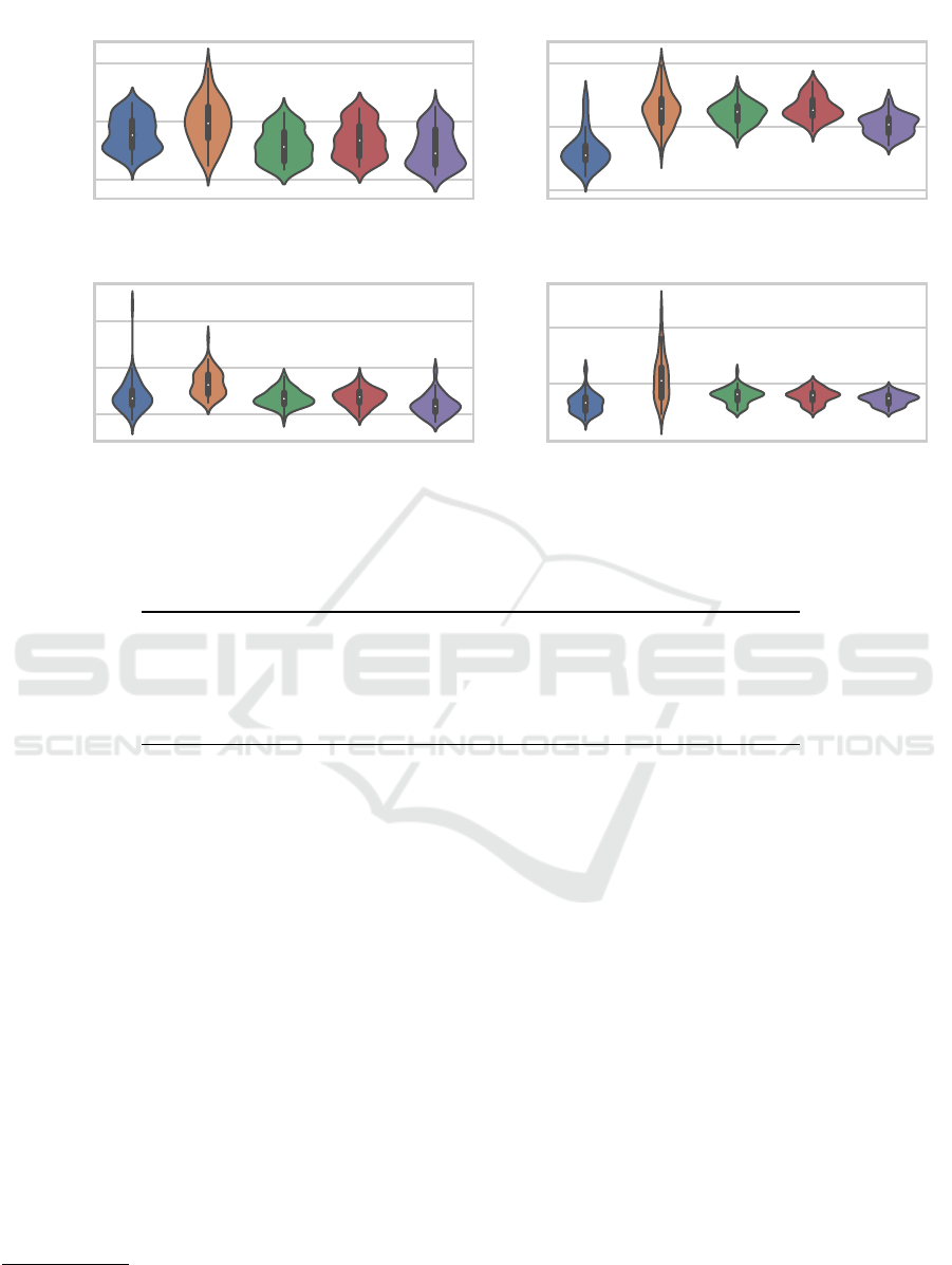
visualize the MSE results (Figure 1). It can be seen
that, on CCPP (top left in Figure 1), the distributions
of MSE values achieved look very similar, with NS
and NSLC maybe having a very slight edge (consider
the y axis scale) which is not visible in the rounded
mean and standard deviations given in Table 2. For
the ASN dataset, the corresponding violin plot (top
right in Figure 1) as well as the values in Table 2
suggest that ES outperforms the other optimizers and
NSLC is slightly better than NS and MCNS. How-
ever, with respect to model complexity (Table 3), we
observe inverse results: NS and MCNS depict a sim-
ilarly low model complexity, while the mean number
of rules in the solutions found by NSLC, ES and RS
is higher by more than ten. When regarding the CS
dataset, Table 2 and Figure 1 (bottom left) hint to-
wards NSLC being the best of the considered meth-
ods with ES, NS and NSLC performing similarly to
each other but slightly worse than NSLC. In terms of
model complexity (Table 3), this is, again, reversed:
ES, NS and MCNS are similar once more and re-
sult in less complex solutions than NSLC. For the
last dataset, EEC, ES is indicated again as the best
performing method (bottom right in Figure 1). The
Approaches for Rule Discovery in a Learning Classifier System
43
ES RS NS MCNS NSLC
0.06
0.07
0.08
CCPP
ES RS NS MCNS NSLC
0.1
0.2
0.3
ASN
ES RS NS MCNS NSLC
RD method
0.1
0.2
0.3
MSE
CS
ES RS NS MCNS NSLC
0.00
0.05
0.10
EEC
Figure 1: Standardized (per task) mean squared errors (MSEs) achieved by the different RD methods on the different tasks.
Table 2: Mean and standard deviation (over 64 runs, rounded to two decimal places) of MSE achieved by the five RD
approaches on the four datasets. Best entry in each row (if one exists) marked in bold.
ES RS NS MCNS NSLC
CCPP 0.07 ± 0.00 0.07 ± 0.00 0.07 ± 0.00 0.07 ± 0.00 0.07 ± 0.00
ASN 0.16 ± 0.03 0.23 ± 0.03 0.22 ± 0.02 0.23 ± 0.02 0.20 ± 0.02
CS 0.14 ± 0.04 0.17 ± 0.03 0.13 ± 0.02 0.13 ± 0.02 0.12 ± 0.02
EEC 0.03 ± 0.01 0.06 ± 0.02 0.04 ± 0.01 0.04 ± 0.01 0.04 ± 0.01
model complexity, however, is lower for NSLC and
much lower for NS and MCNS.
Overall, the visual analysis combined with the
rounded statistics of mean and standard deviation
are not capable of providing us with a conclusive
answer regarding which of the RD methods should
be preferred on tasks like the ones considered. We
thus investigate the data gathered more closely using
Bayesian data analysis
2
.
We start by applying to our data the model pro-
posed by Calvo et al. (Calvo et al., 2018; Calvo et al.,
2019) which, for each of the RD methods, provides
us with the posterior distribution over the probabil-
ity of that RD method performing best. We apply this
model to both the MSE observations as well as the
model complexity observations and provide box plots
(Figures 2 and 3) which show the most relevant distri-
bution statistics. Both figures show that the distribu-
tions over the probabilities of performing the best are
rather tight. However, the figures also show that there
2
We deliberately do not use null hypothesis signifi-
cance tests due to their many flaws and possible pitfalls—cf.
e.g. (Benavoli et al., 2017).
cannot be made a very confident conclusive statement
for a single RD method given the data available: For
both metrics, the highest expected value for the proba-
bility of being the best assigned by the model to a sin-
gle RD method is only around 40 % (to illustrate: this
means that the probability of that candidate not being
the best is around 60 %). Due to this, we also consid-
ered the probability distribution over the probability
of either ES or NSLC performing the best MSE-wise
since those were the highest probability candidates
with respect to that metric. As can be seen, for MSE,
the probability of either of the two being ranked the
best is still merely around 60 % which still does not
amount to much evidence. Only if we include the top
three options (ES, NSLC and NS), are we entering the
region of over 80 % where we could say with some
slight confidence that the best-performing is among
those three.
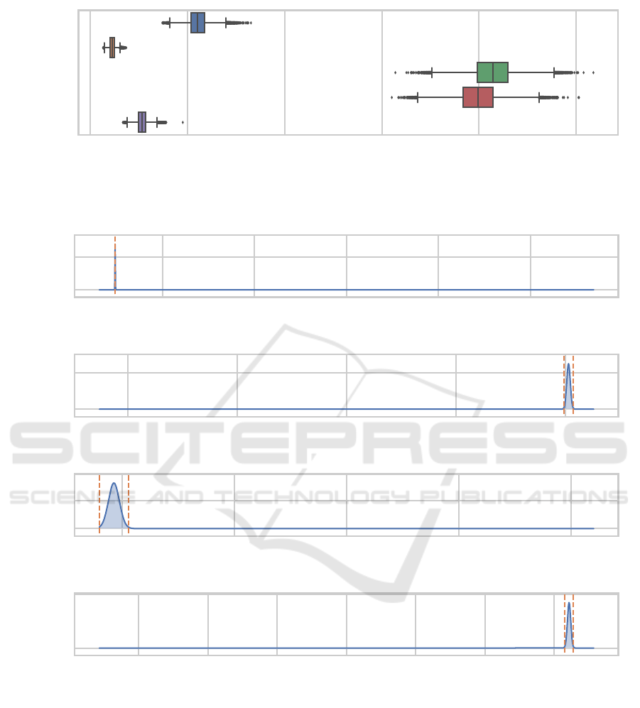
When considering model complexity (Figure 3),
there is an 80 % probability that one of NS and MCNS
performs the best. However, since the probability of
each of these not performing the best MSE-wise is
around 80 % or more, we do not consider them to be
ECTA 2022 - 14th International Conference on Evolutionary Computation Theory and Applications
44
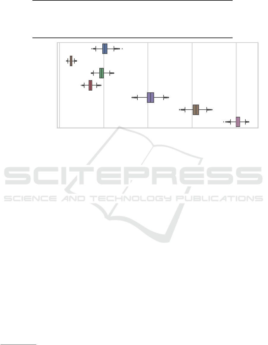
Table 3: Mean and standard deviation like Table 2 but for model complexity.
ES RS NS MCNS NSLC
CCPP 04.52 ± 1.48 12.86 ± 3.13 05.84 ± 0.91 06.02 ± 1.39 06.94 ± 1.41
ASN 31.78 ± 2.21 32.98 ± 3.11 18.22 ± 2.91 18.81 ± 2.46 29.75 ± 3.84
CS 24.95 ± 2.45 29.56 ± 2.47 23.50 ± 3.47 22.38 ± 3.02 33.83 ± 3.28
EEC 12.94 ± 2.10 30.17 ± 3.78 06.92 ± 1.70 06.22 ± 1.13 10.16 ± 1.94
0.0 0.2 0.4 0.6 0.8
Probability
ES
RS
NS
MCNS
NSLC
ES ∧ NSLC
ES ∧ NSLC ∧ NS
RD method
Figure 2: Box plot (with standard 1.5 IQR whiskers and outliers) of the posterior distribution obtained from the model by
Calvo et al. (Calvo et al., 2018; Calvo et al., 2019) applied to the MSE data. An RD method having a probability value of q %
says that the probability of that RD method performing the best with respect to MSE is q %. In addition to each individual
RD method we also included the distributions for “either of ES or NSLC (or NS) perform best”.
competitive enough to merit a closer analysis within
the present work.
We next consider the difference in performance
between ES (since it is both the originally-used RD
method as well as the runner-up with respect to
the probability of being the best MSE-wise) and
NSLC (since it has the highest probability of hav-
ing the lowest MSE) by applying Corani and Be-
navoli’s Bayesian correlated t-test (Corani and Be-
navoli, 2015). The resulting posteriors (given in Fig-
ures 4 and 5 including 99 % HDIs) are the distribution
of the difference between the considered metric for
NSLC and the considered metric for ES (which means
that values larger than zero indicate NSLC having a
higher (worse) metric value than ES). It can be seen
that, on the CCPP dataset, the difference in MSEs be-
tween NSLC and ES is most certainly negligible in
practice which corroborates the earlier statement that
on that dataset all but RS perform similarly. On ASN,
on the other hand, ES outperforms NSLC by an MSE
of at least 0.04 with a probability of over 99 %
3
(99 %
of probability mass already lies between the dashed
lines alone and even more to the right the upper HDI
bound). The probability of NSLC outperforming ES
3
This means that in over 99 % of future runs we would
expect the MSE difference between the two approaches to
be at least 0.04.
on the CS dataset by an MSE of 0.019 to 0.022 is
99 %. On EEC, the last of the four datasets, there
is, again, not really a significant difference to be no-
ticed (e.g. if a difference in MSE of 0.0033 could be
considered not practically relevant on this dataset then
the two should be considered to perform equivalently
with a probability of over 99 %).
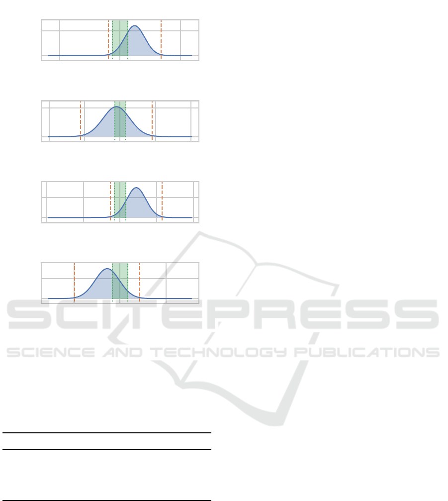
Things look differently when regarding the model
complexities produced by the two approaches (Fig-
ure 5). On each of the datasets, there is considerable
probability mass on each side of 0. While we could
simply compute the integral to the left (or right) of 0,
this would include differences that are not relevant in
practice. We thus decided to define a region of prac-
tical equivalence (rope) centered on a complexity dif-
ference of 0. Since the learning tasks are very dif-
ferent in their model complexity (i.e. require different
solution sizes), we opted for a task-dependent rope.
As this is difficult to choose based on the task alone
(i.e. requiring detailed domain knowledge about the
different processes that generated the data), we let the
collected data inform our choice of the rope for each
task: We choose as the bounds of the rope the mean of
the standard deviations of ES, NS, MCNS and NSLC
(leaving out RS since that method does not even re-
motely achieve competitive results with respect to so-
lution complexity). The rope for each task is included
Approaches for Rule Discovery in a Learning Classifier System
45
0.0 0.1 0.2 0.3 0.4 0.5
Probability
ES
RS
NS
MCNS
NSLC
RD method
Figure 3: Box plot like Figure 2 but for the model complexity metric.
−0.002 −0.001 0.000 0.001 0.002
0
50000
-0.0025-0.0025
CCPP
−0.04 −0.02 0.00 0.02 0.04
0
1000
0.04 0.041
ASN
−0.02 −0.01 0.00 0.01 0.02
0
500
-0.022 -0.019
CS
−0.003 −0.002 −0.001 0.000 0.001 0.002 0.003
MSE(NSLC) - MSE(ES)
0
20000
Density
0.0032 0.0033
EEC
Figure 4: Density plot of the posterior distribution obtained from Corani and Benavoli’s Bayesian correlated t-test (Corani
and Benavoli, 2015) applied to the difference in MSE between NSLC and ES. Orange dashed lines and numbers indicate the
99 % HDI (i.e. 99 % of probability mass lies within these bounds). HDI bounds rounded to two significant figures.
in Figure 5 as a green area delimited by green dotted
lines. Based on the rope and the Bayesian correlated
t-test model we can now compute the probabilities for
ES and NSLC performing practically equivalently or
worse than the other; they are given in Table 4. Upon
close inspection we can determine that for ASN, the
data is not conclusive. For CCPP and CS, ES pro-
duces less complex solutions than NSLC with a prob-
ability of 75.1 % and 86.2 % respectively. For EEC
there is some evidence hinting towards NSLC creat-
ing more compact solutions, however, this, again is
not fully conclusive as the probability of this not be-
ing the case is 34.4 %.
We conclude our analysis with a summary of the
key takeaways.
ECTA 2022 - 14th International Conference on Evolutionary Computation Theory and Applications
46
−10 0 10
0.0
0.2
-2.0 6.8
CCPP
−40 −20 0 20 40
0.00
0.05
-22.0 18.0
ASN
−40 −20 0 20 40
0.00
0.05
-5.1 23.0
CS
−10 0 10
Model complexity(NSLC)
- Model complexity(ES)
0.0
0.1
Density
-9.9 4.3
EEC
Figure 5: Density plot like Figure 4 but for the model com-
plexity metric and with the region of practical equivalence
(rope) marked by green dotted lines and a green area.
Table 4: Probability (in percent, rounded to one decimal
place) of ES or NSLC performing better or worse than the
other—or practically equivalently—with respect to model
complexity.
ES worse pract. equiv. NSLC worse
CCPP 1.3 23.5 75.1
ASN 45.6 28.4 26.0
CS 1.4 12.4 86.2
EEC 65.6 29.6 4.9
• NSLC has the highest probability of being the
best option MSE-wise on datasets like the ones
we considered. However, the data we collected is
not entirely conclusive with respect to that (there
is still an around 60 % chance of NSLC not having
the best MSE on such datasets).
• When considering model complexity alone, there
is a high probability of either of NS or MCNS
being the best—however, their MSEs are with a
high probability not the best.
• A closer comparison of ES with NSLC yielded:
– ES outperforms NSLC MSE-wise with very
high probability (> 99 %) by a presumably
practically relevant amount on ASN whereas
this is the other way around on CS. However,
on these two tasks, the data is either not con-
clusive as to which method yields the better
model complexities (ASN) or the method with
the worse MSE performs better in that regard
(CS).
– On the other two tasks, ES and NSLC per-
form somewhat equivalently MSE-wise. There
is some light evidence for ES yielding better
model complexities on the less difficult of these
(CCPP) and for NSLC yielding better model
complexities on the more difficult one (EEC).
• Overall, we can say that despite its simplic-
ity when compared to the other approaches, the
(1,λ)-ES performs not worse when only consid-
ering practically relevant differences.
5 CONCLUSION
This work investigated the use of different evolution-
ary approaches towards rule discovery in the Super-
vised Rule-based learning system (SupRB), a recently
proposed Learning Classifier System (LCS) for re-
gression problems. This system’s key characteristic
is the separation of finding a diverse pool of rules that
fit the data well from their composition into a model
that is both accurate and uses a minimal number of
rules—a key advantage when employed in settings
where model transparency is important, such as typi-
cal explainable artificial intelligence applications. By
determining from intermediate solutions which areas
of the problem space were already well covered, sub-
sequent evolution can be guided towards other areas
to form new rules there and, therefore, improve the
overall diversity of the available rules.
The investigated methods were a (1,λ)-ES, a Ran-
dom Search (RS) and three Novelty Search (NS) vari-
ants. The NS-based variants all employed a (µ,λ)-
ES, scored a rule’s novelty on the basis of its match
set and combined it with traditional fitness. Besides a
traditional NS, we investigated Minimal Criteria Nov-
elty Search (MCNS) and Novelty Search with Local
Competition (NSLC).
After an evaluation of the five methods on four
real-world regression problems, we found that perfor-
mances are similar but, depending on the dataset, spe-
cific methods can be preferred, with ES and NSLC
Approaches for Rule Discovery in a Learning Classifier System
47

being the most interesting candidates. This was con-
firmed by a rigorous statistical analysis. Interestingly,
we found that where ES can be expected to perform
better on error than NSLC, it can also be expected to
yield larger solution sizes (a higher number of rules
in the model) and vice versa.
Overall, we recommend to use either ES or NSLC,
although, due to its greater simplicity and the fact that
rules are selected independently of the status of other
rules, ES seems to be the preferential candidate for
cases where model construction is important for the
explainability requirements of users.
ACKNOWLEDGEMENTS
This work was partially funded by the Bavarian Min-
istry of Economic Affairs, Energy and Technology.
REFERENCES
Akiba, T., Sano, S., Yanase, T., Ohta, T., and Koyama,
M. (2019). Optuna: A Next-generation Hyperpa-
rameter Optimization Framework. In Proceedings
of the 25th ACM SIGKDD International Conference
on Knowledge Discovery & Data Mining, KDD ’19,
pages 2623–2631, New York, NY, USA. Association
for Computing Machinery.
Benavoli, A., Corani, G., Dem
ˇ
sar, J., and Zaffalon, M.
(2017). Time for a change: A tutorial for compar-
ing multiple classifiers through bayesian analysis. J.
Mach. Learn. Res., 18(1):2653–2688.
Brooks, T., Pope, D., and Marcolini, M. (1989). Airfoil
Self-Noise and Prediction. Technical Report RP-1218,
NASA.
Calvo, B., Ceberio, J., and Lozano, J. A. (2018). Bayesian
inference for algorithm ranking analysis. In Proceed-
ings of the Genetic and Evolutionary Computation
Conference Companion, GECCO ’18, pages 324–325,
New York, NY, USA. Association for Computing Ma-
chinery.
Calvo, B., Shir, O. M., Ceberio, J., Doerr, C., Wang, H.,
B
¨
ack, T., and Lozano, J. A. (2019). Bayesian per-
formance analysis for black-box optimization bench-
marking. In Proceedings of the Genetic and
Evolutionary Computation Conference Companion,
GECCO ’19, pages 1789–1797, New York, NY, USA.
Association for Computing Machinery.
Corani, G. and Benavoli, A. (2015). A bayesian approach
for comparing cross-validated algorithms on multiple
data sets. Machine Learning, 100(2):285–304.
Dua, D. and Graff, C. (2017). UCI machine learning repos-
itory. http://archive.ics.uci.edu/ml.
Gomes, J., Mariano, P., and Christensen, A. L. (2015). De-
vising effective novelty search algorithms: A com-
prehensive empirical study. In Proceedings of the
2015 Annual Conference on Genetic and Evolution-
ary Computation, GECCO ’15, page 943–950, New
York, NY, USA. Association for Computing Machin-
ery.
Gomes, J., Urbano, P., and Christensen, A. L. (2012). Pro-
gressive minimal criteria novelty search. In Pav
´
on,
J., Duque-M
´
endez, N. D., and Fuentes-Fern
´
andez,
R., editors, Advances in Artificial Intelligence – IB-
ERAMIA 2012, pages 281–290. Springer Berlin Hei-
delberg.
Heider, M., Nordsieck, R., and H
¨
ahner, J. (2021). Learn-
ing Classifier Systems for Self-Explaining Socio-
Technical-Systems. In Stein, A., Tomforde, S., Botev,
J., and Lewis, P., editors, Proceedings of LIFELIKE
2021 co-located with 2021 Conference on Artificial
Life (ALIFE 2021).
Heider, M., Stegherr, H., Nordsieck, R., and H
¨
ahner,
J. (2022a). Learning classifier systems for self-
explaining socio-technical-systems. https://arxiv.org/
abs/2207.02300. Submitted as an extended version of
(Heider et al., 2021).
Heider, M., Stegherr, H., Wurth, J., Sraj, R., and H
¨
ahner, J.
(2022b). Separating Rule Discovery and Global So-
lution Composition in a Learning Classifier System.
In Genetic and Evolutionary Computation Conference
Companion (GECCO ’22 Companion).
Heider, M., Stegherr, H., Wurth, J., Sraj, R., and H
¨
ahner, J.
(2022c). Investigating the impact of independent rule
fitnesses in a learning classifier system. http://arxiv.
org/abs/2207.05582. Accepted for publication in the
Proceedings of BIOMA’22.
Kaya, H. and T
¨
ufekci, P. (2012). Local and Global Learn-
ing Methods for Predicting Power of a Combined Gas
& Steam Turbine. In Proceedings of the Interna-
tional Conference on Emerging Trends in Computer
and Electronics Engineering ICETCEE.
Lehman, J. (2012). Evolution Through the Search for Nov-
elty. PhD thesis, University of Central Florida.
Lehman, J. and Stanley, K. O. (2010). Revising the evo-
lutionary computation abstraction: Minimal criteria
novelty search. In Proceedings of the 12th Annual
Conference on Genetic and Evolutionary Computa-
tion, GECCO ’10, page 103–110, New York, NY,
USA. Association for Computing Machinery.
Pedregosa, F., Varoquaux, G., Gramfort, A., Michel, V.,
Thirion, B., Grisel, O., Blondel, M., Prettenhofer, P.,
Weiss, R., Dubourg, V., Vanderplas, J., Passos, A.,
Cournapeau, D., Brucher, M., Perrot, M., and Duch-
esnay,
´
E. (2011). Scikit-learn: Machine Learning in
Python. The Journal of Machine Learning Research,
12:2825–2830.
Tsanas, A. and Xifara, A. (2012). Accurate Quantitative Es-
timation of Energy Performance of Residential Build-
ings Using Statistical Machine Learning Tools. En-
ergy and Buildings, 49:560–567.
T
¨
ufekci, P. (2014). Prediction of full load electrical power
output of a base load operated combined cycle power
plant using machine learning methods. Interna-
tional Journal of Electrical Power & Energy Systems,
60:126–140.
ECTA 2022 - 14th International Conference on Evolutionary Computation Theory and Applications
48

Urbanowicz, R. J. and Browne, W. N. (2017). Introduction
to Learning Classifier Systems. Springer Publishing
Company, Incorporated, 1st edition.
Urbanowicz, R. J. and Moore, J. H. (2009). Learning Clas-
sifier Systems: A Complete Introduction, Review, and
Roadmap. Journal of Artificial Evolution and Appli-
cations.
Wilson, S. W. (1995). Classifier fitness based on accuracy.
Evolutionary Computation, 3(2):149–175.
Wurth, J., Heider, M., Stegherr, H., Sraj, R., and H
¨
ahner, J.
(2022). Comparing different metaheuristics for model
selection in a supervised learning classifier system.
In Genetic and Evolutionary Computation Conference
Companion (GECCO ’22 Companion).
Yeh, I.-C. (1998). Modeling of Strength of High-
Performance Concrete Using Artificial Neural Net-
works. Cement and Concrete Research, 28(12):1797–
1808.
Approaches for Rule Discovery in a Learning Classifier System
49
