A MLP for Dryer Energy Consumption Prediction in Wood Panel

Industry

Valentin Chazelle

1,2 a

, Philippe Thomas

1 b

and Hind Bril El-Haouzi

1 c

and Christophe Heleu

CRAN, Universit

e de Lorraine, CNRS, 27 rue Philippe Seguin, 88800 Epinal, France

Egger Panneaux & Decors, 88700 Rambervillers, France

Keywords:

MLP Neural Network, Energy Consumption Prediction, Wood Panel Industry, Industrial Dryer.

Abstract:

The drying operation is the most energy consuming step of particle board manufacturing process. Even if a

great academic and industrial effort has been furnished for last years, the prediction of this energy consumption

is still a challenging issue. This paper deals with the energy consumption prediction for industrial wood

drying. The study of an European particle board manufacturer’s industrial dryers has provided data sets for

two both fresh and recycled wood drying processes. Based on these, MLP Neural network models have been

developed and tested. Several tests have been conduced to identify and select the best MLP model’s structure

to ﬁnd a satisfying trade-off between model accuracy and maintenance efﬁciency. The proposed MLP models

have either been distinctly trained on the datasets from both the ﬁrst and second dryers, and then on their

combination, in order to increase data diversity and to reduce training time and model maintenance. Then, the

neural network based on the merged dataset has been compared to those developed from the single datasets.

This experiment led to the conclusion that, the construction of a global model representing the operation of the

two dryers is less accurate than the construction of a dedicated model for each dryer. Yet, the performances of

combination model remain acceptable.

1 INTRODUCTION

The wood panel industry has a great socio-economic

importance at both European and French scales. In

2019, the European production of all the manufac-

turers in the sector was representing 76.4 million m

of panels

, 22 billions euros, and 100,000 jobs. In

France alone, the overall turnover is more than 1.2

billion euros and the sector directly employs around

3,000 people

Particle boards being commodity products, their

price is a major factor for customers’ purchasing

decision-making. Therefore producers strive to pro-

duce at the lowest possible cost. Yet, these costs

are dependent on many variables, such as raw mate-

rial availability and prices (generally related), quality

speciﬁcations, or equipment capacities & energy con-

https://orcid.org/0000-0001-9496-0907

https://orcid.org/0000-0001-9426-3570

https://orcid.org/0000-0003-4746-5342

https://europanels.org/

http://www.uipp.fr/

sumption (Buehlmann et al., 2000). Due to the large

amount of potential variables involved, ﬁnding an op-

timal solution by simulation or any other empirical

technique is almost impossible.

The rise of Industry 4.0 (Lasi et al., 2014) and its

associated technology (smart materials and sensors,

IoT, etc.) opens the opportunity to collect and ex-

ploit the huge amount of data created by industrial

processes. Also, it makes credible the modelling of

complex systems, for instance to predict machines’

behaviours. Explorations and using these data will

certainly help improving processes efﬁciency and re-

sources consumption in industry at very short term.

The drying operation is the most energy consum-

ing step of particle boards manufacturing process.

Also, the drying mechanisms involve elements of dif-

ferent sizes (barks, sawdust...) and the dryer perfor-

mance is seen according to a macroscopic view. Due

to lack of sustainable link between these two scales,

the drying operation is the most difﬁcult part to model

(Huang and Mujumdar, 1993). In woods industry,

Chazelle, V., Thomas, P., El-Haouzi, H. and Heleu, C.

A MLP for Dryer Energy Consumption Prediction in Wood Panel Industry.

DOI: 10.5220/0011541900003332

In Proceedings of the 14th International Joint Conference on Computational Intelligence (IJCCI 2022), pages 381-388

ISBN: 978-989-758-611-8; ISSN: 2184-2825

381

drying consists in lowing moisture

content of wood

material to the required level for the process and the

quality of ﬁnal product. Therefore, the cost of this

operation is highly linked to the price of energy. In

addition, the moisture content of raw wood changes

according to seasons and types of wood, making the

drying operation difﬁcult to optimise. As a critical

operation, drying is nowadays automated and mon-

itored, and key parameters are recorded and stored.

This collected database enables the modelling of the

dryer to reproduce its energy consumption behaviour

depending on the raw mix product, the moisture and

the mass ﬂow. To model the dryer itself, several op-

tions, such as linear or nonlinear modeling, could be

considered. In the past, neural networks have often

been successfully used to model dryers, with different

goals. For the conception, a 3 layers neural network

was used to predict off-design performance of dryers

(exit temperature and moisture) (Huang and Mujum-

dar, 1993). To increase accuracy of control system

of a continuous grain dryer, (Jin et al., 2021) use a

Neural Network to model the dryer. In their study,

(Azadbakht et al., 2016) have worked on predicting

the parameters of energy and exergy analysis for dry-

ing of potatoes for food industry. Their results suggest

that neural networks can help to optimize the use of

energy during the drying process. In wood industry,

MLP was used to model a sawmill workshop, in or-

der to reduce bottleneck (Thomas and Thomas, 2011).

Also, MLP are used to make lumber production pre-

diction in sawmill (Martineau et al., 2021). For this

reason, nonlinear modeling with multilayers percep-

tron (MLP) network will be used in this paper.

In the industry, models have to be maintained to

keep up with changing reality. In this context, main-

taining one model instead of several is easier and

cheaper. In this spirit, the main objective of this paper

is to evaluate the beneﬁts of combining the databases

of the two dryers, in order to increase the diversity of

databases (different operating points) and evaluate the

impact on the quality of predictions.

The remaining of this paper is structured as fol-

lows: The ﬁrst part presents a preliminary study of

related works. Then, the process of wood dryers are

presented in section 2, and the approach is in section

3. This will be followed by the experimental results in

section 4. Section 5 concludes this paper and presents

future avenues for work and reﬂection.

In wood particles boards, wet mass to dry mass.

2 PROCESS OF WOOD DRYERS

To better understand the model parameters and their

impacts, the indirect steam-tube dryer needs to be pre-

sented, followed by the presentation of the recording

data from these dryers.

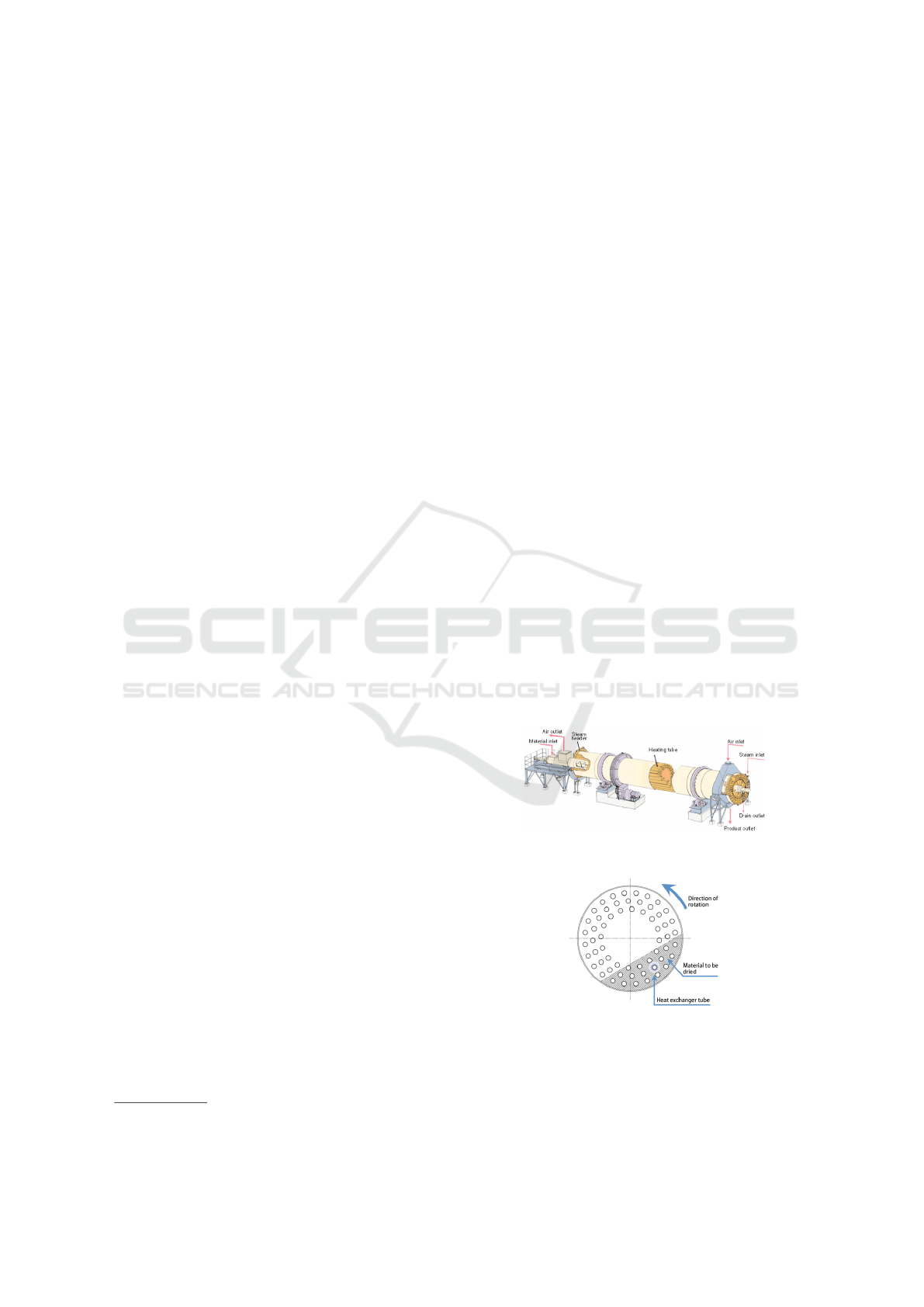
In this application case, two parallel indirect

steam-tube dryers are used to dry the wet raw wood

supplied. An indirect steam-tube dryer is a rotating

cylinder heated to 150°C into which wet material is

continuously fed on one side and dry material exit on

the other (ﬁgure 1). Heat is supplied by steam. There

is no contact between the steam and the wet material

(ﬁgure 2). In the steam network there are three parts,

one heat exchanger to warm the incoming air, and two

tubes: one in entry of the cylinder and the second in

exit. The ﬁrst tube is used all the time, the second is

used when the raw material contains a high level of

moisture. At the opposite, the exchanger is used only

in winter. In this paper, we focus on data from the two

tubes of each dryer. In the considered case, the two

dryers used different raw materials. Dryer 1 is used

to dry fresh wood (Softwood, hardwood log, chips,

shaving, sawmill residuals and saw dust), which con-

tains a high level of moisture (up to 140%). Dryer 2

is used to dry recycling wood (coming of old furni-

ture and non-treated carpentry), who contains a lower

level of moisture (around 35%). The target output

moisture for these two dryers is less than 5%. Due

to the difference of moisture between the raw mate-

rial (fresh wood and recycling wood), the steam con-

sumption of these two dryers is very different.

Figure 1: Steam Tube Rotary Dryer Components.

Figure 2: Steam Dryer Section.

For the two dryers, the daily’s data recorded over

1.5 years, gives an uncleaned database of 532 lines.

Each line contains two parts, for the raw material (av-

erage per day): the mass ﬂow, the moisture of incom-

NCTA 2022 - 14th International Conference on Neural Computation Theory and Applications

382

ing and the moisture of outgoing. For each dryer, the

data are steam power (in kWh) for the three sections,

Tubes 1 and 2 and exchanger (not used here).

3 PROPOSAL APPROACH

This section will explicit the methodology. The ﬁrst

part concerns the cleaning of database in order to

avoid problems during learning, then the standardi-

sation of the databases, and the datasets creation.

The recording databases presented previously are

uncleaned, they contain registration errors, and sen-

sor measurement faults. The cleaning process con-

tains two steps. The ﬁrst step consists to delete the

line if one variable is empty or missing. This opera-

tion reduces data from 531 lines to 500 for Dryer 1,

and from 531 to 527 for Dryer 2. The second step is

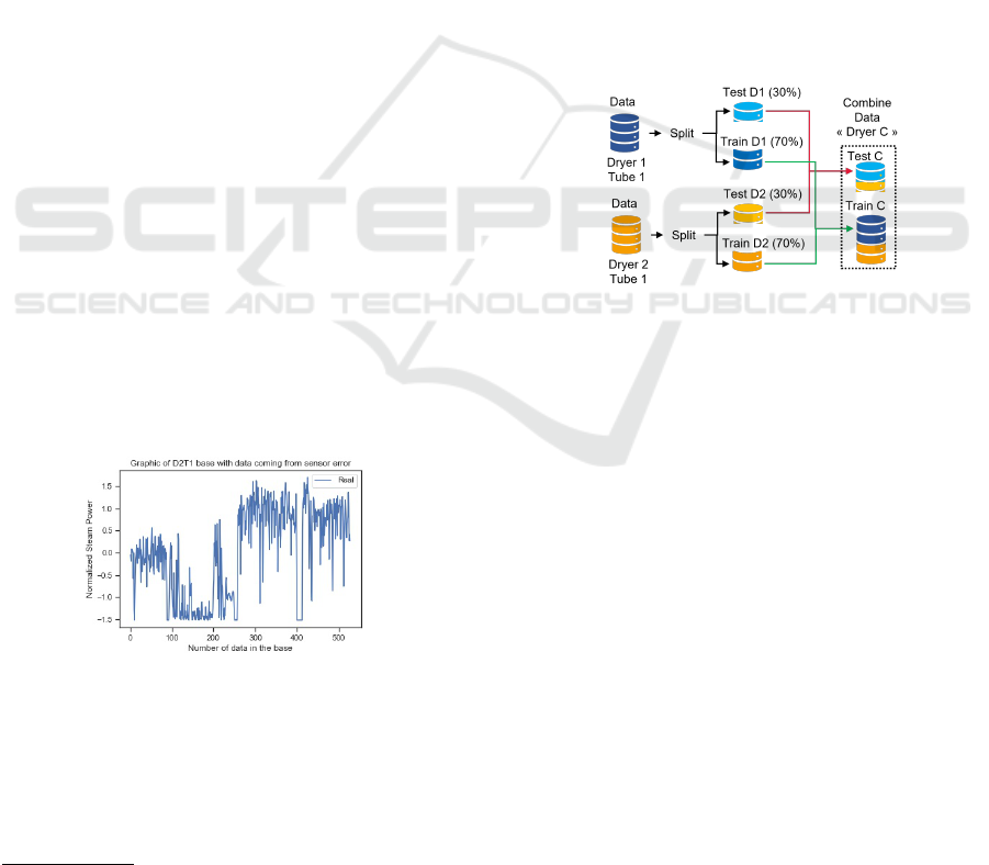
the study of data in chronological order, to detect if

some event occurs. As a result, the tube 1 of dryer

2 looks a bit different as the others, as shown in ﬁg-

ure 3. The difference of level for values before indice

100 and after indice 250 are explained by the season-

ality (summer/winter), who affects the humidity and

temperature of input material. Values between indices

100 and 250 appear very low for this season and after

exchange with dryer management operator, it appears

that the steam sensor, after maintenance, was not put

back in place according to the manufacturer’s recom-

mendation, and the calibration was wrong. These val-

ues are false, so they are deleted from database. Also,

values around index 400 was deleted, they correspond

to a heavy maintenance in the dryer and system was

still recording. All of these deleted values bring the

database of dryer 2 tube 1 to 386 lines.

Figure 3: Dryer 2 Tube 1: Effect of sensor Fail in recording

steam power.

After the cleaning of the database, a standardisa-

tion of the data must be performed to improve the ac-

curacy of the learning. All variables (inputs and out-

put) of the databases are standardized using the stan-

dard scaler from python

. The standard score z of a

https://scikit-learn.org/stable/modules/generated/

sklearn.preprocessing.StandardScaler.html

sample x is calculated as equation 1:

z = (x − u)/s (1)

where u is the mean of the sample x, s is the standard

deviation of x.

There are two dryers and each dryer have two

tubes. So, there are 4 databases. To allow the learn-

ing of the models, these databases must be split into

learning (70% of data) and validation datasets (30%

of data). The main goal of this paper is to evalu-

ate if it is better to build one model for each dryer

or one model common for the two dryers. Thereby,

datasets (for learning and validation) related to tube 1

from dryers 1 and 2 are combined (same process for

tube 2). Figure 4 shows the combination method de-

scribed above for tube 1. The new datasets are stored

as a dryer ”Combination” (”C”). So, at the end of this

stage, there is 6 databases, each of them is split into

train and test datasets: Dryer 1 Tube 1, Dryer 1 Tube

2, Dryer 2 Tube 1, Dryer 2 Tube 2, and the combina-

tion of them in Dryer C Tube 1, Dryer C Tube 2.

Figure 4: Process of combination data and creation ”Dryer

C”.

At this stage, the metamodel must be chosen. The

choice fells on a multilayers perceptron (MLP) in-

cluding only one hidden layer and one output neu-

ron. Output neuron activation function is linear, and

the hidden neurons have an hyperbolic tangent ac-

tivation function. This MLP is chosen because it

has been proved that it is an universal approxima-

tor and it has been succesfully used to model dry-

ers in the past (Huang and Mujumdar, 1993), (Jin

et al., 2021) and (Azadbakht et al., 2016). The in-

put layer includes 3 neurons. The initialisation is

performed by using Nguyen and Widrow algorithm

(Nguyen and Widrow, 1990). The learning is per-

formed by using an hessian backpropagation algo-

rithm, the Levenberg-Marquardt algorithm (Sapna,

2012) which presents the advantage to speed up the

convergence of the learning particularly for the small

datasets.

The structure of the MLP is not yet totally de-

ﬁned. The number of hidden neurons must be ﬁxed.

To do that, for each model, ﬁfteen conﬁgurations of

neural network are trained, with a number of hidden

A MLP for Dryer Energy Consumption Prediction in Wood Panel Industry

383

neurons varying between 1 and 15. To avoid local

minimum trapping problem, for each conﬁguration,

two hundred different initialization sets are drawn be-

fore training is performed. Learning continues un-

til there is no progression of the Root Mean Square

Error (RMSE) calculated on the learning dataset (up

to ﬁve thousand iterations). For each conﬁguration

the model (among the two hundred different) with the

lowest RMSE on the train dataset is selected.

To determine the best structure, the ﬁfteen mod-

els selected (for the different conﬁgurations) are com-

pared with their RMSE on the validation dataset. Sta-

tistical tests are also performed. Finally, for each tube,

three models are selected and compared. These three

models are built by using databases related to dryers

1, 2 and combined respectively.

4 RESULTS

In this section, the procedure used to build and com-

pare models for the two tubes is described. First the

structure determination must be performed, then the

three selected models are compared. ”NNC” cor-

responds to neural network learned on dataset from

Dryer Combination (coming from the combination of

datasets from Dryers 1 and 2). ”NN1” and ”NN2”

correspond respectively to neural network learned on

datasets from Dryer 1 (D1) and from Dryer 2 (D2).

So, for each Tube, there is 2 NN possible: ”NNC” or

”NN1” for Dryer 1, and ”NNC” or ”NN2” for Dryer

2. The design of the different models for Tube 1 (T1)

is the ﬁrst to be presented, Followed by tube 2 (T2).

4.1 Model Selection

4.1.1 Tube 1

For the Tube 1, the best conﬁguration for each model

is determined in this section.

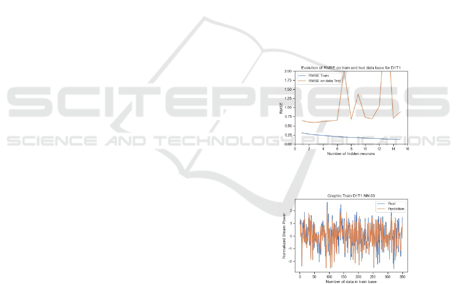
Dataset Dryer 1. For NN applied on Dryer 1 Tube

1 the RMSE on train dataset are decreasing from 0.31

for 1 neuron to 0.12 for 15 neurons (table 1). Figure

5 shows the evolution of RMSE on training and test

datasets. As expected, the increasing of number of

neurons decreases the RMSE and increases the qual-

ity of prediction on training dataset. For the RMSE

on test dataset, the lowest point is reached with 3 neu-

rons, at the value of 0.59, and RMSE increases after

this point, as shown ﬁgure 5. This fact was expected

because the selection of the best model (among the

two hundred) is performed on the train dataset and so,

the overﬁtting problem occurs allowing to identify the

optimal structure (here 3 hidden neurons).

Figure 6 shows the real values and the ”T1 NN1

3” prediction values of the energy consumption for

the train dataset. This ﬁgure shows that these two

curves are closed to each other. Figure 7 presents the

same values but for the test dataset. It appears that the

model ”T1 NN1 3” can reach all the points in the test

dataset and have not inconsistent values. This fact is

conﬁrmed by the regression graphic given ﬁgure 8.

For this reason, the conﬁguration with 3 neurons

(”T1 NN1 3”) is chosen as reference for a khi-2 test,

to ﬁnd if there is a statistical difference between this

model and the other conﬁgurations. The khi-2 hy-

pothesis tests (table 1) show that conﬁguration 1 to 6

(”T1 NN1 1” to ”T1 NN1 6”) are not statically dif-

ferent from ”T1 NN1 3”. According to the results

of these tests, ”T1 NN1 1” can be chosen to reduce

number of neurons. However, when comparing accu-

racy of models ”T1 NN1 1” and ”T1 NN1 3” on train

dataset, it appears that ”T1 NN1 3” is statistically bet-

ter than ”T1 NN1 1”. That’s why the model ”T1 NN1

3” is selected for the following.

Figure 5: T1 NN1: Evolution of RMSE on train and test

datasets, function of number of hidden neurons.

Figure 6: T1 NN1 3: Real and Prediction Values on Train

datasets on Tube 1 Dryer 1.

Dataset Dryer 2. The same work performed for

dryer 1 Tube 1 is applied on Dryer 2 Tube 1. The

results are summarized ﬁgure 9 which presents the

evolve of RMSE in function of the hidden neurons

number for train and test datasets. For similar reasons

than for dryer 1, the model ”T1 NN2 4” is selected.

The RMSE values of this model for the train and test

datasets are 0.15 and 0.43 respectively.

NCTA 2022 - 14th International Conference on Neural Computation Theory and Applications

384

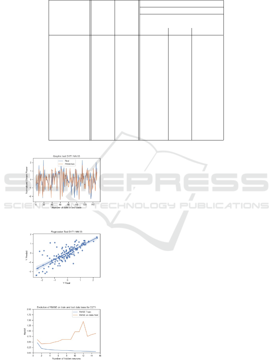
Table 1: T1 NN1 apply to Dryer 1 (RMSE on train and Test datasets, Γ and Hypothesis testing).

Conﬁguration Test basis: 150

and Degree of freedom: 149

Number of RMSE RMSE Γ

lower

= 117.10

hidden on on Γ

upper

= 184.69

neurons Train Test Taux Γ Pvalue Result

1 0.31 0.64 175.42 0.069 Accept

2 0.27 0.60 152.63 0.402 Accept

3 0.25 0.59 - - Reference

4 0.24 0.62 161.20 0.234 Accept

5 0.22 0.63 169.83 0.116 Accept

6 0.21 0.65 179.38 0.045 Accept

7 0.19 2.02 1715.09 0.000 Reject

8 0.18 0.68 1953 0.006 Reject

9 0.18 1.36 785.07 0.000 Reject

10 0.16 0.73 223.01 0.000 Reject

11 0.16 0.70 204.58 0.002 Reject

12 0.15 1.04 452.99 0.000 Reject

13 0.14 3.71 5810.26 0.000 Reject

14 0.14 0.71 212.57 0.000 Reject

15 0.12 0.88 327.21 0.000 Reject

Figure 7: T1 NN1 3: Real and Prediction Values on Test

dataset on Tube 1 Dryer 1.

Figure 8: T1 NN1 3: Regression on test dataset between

Real and Prediction Values.

Figure 9: T1 NNC: Evolution of RMSE on train and test

datasets, function of number of hidden neurons.

Dataset Dryer Combination. ”NNC” is the NN

learned on the dataset of the Dryer C. The same work

performed for the two preceding models is applied on

Dryer C Tube 1. For NN applied on Dryer C Tube 1

the RMSE on train dataset are decreasing from 0.67

for 1 neuron to 0.24 for 15 neurons (table 2). Figure

10 shows the evolution of RMSE on training and test

datasets. For the RMSE on test dataset, the lowest

point is reached with 13 neurons, at the value of 0.66.

Figure 11 presents the regression graphic for the test

dataset. It appears that the model ”T1 NNC 13” can

reach all the points in the test dataset and have not

inconsistent values. The second lowest point is con-

ﬁguration 3 with 0.67. These 2 conﬁgurations look

similar, so to ﬁnd if there is a statistical difference

between them a khi-2 test is performed. According

to the results of this test, ”T1 NNC 3” can be cho-

sen to reduce number of neurons. However, due to

the great difference (statistically signiﬁcant) between

RMSE obtained for the train test for ”T1 NNC 3” and

”T1 NNC 13” on the train dataset, the model ”T1 NN1

13” is chosen for the following.

4.1.2 Tube 2

For the Tube 2, the same procedure is used than pre-

viously.

Dataset Dryer 1. The same work performed for

dryer 1 Tube 1 (ref:4.1.1.1 ) is applied on Dryer 1

Tube 2. The results are summarized ﬁgure 12 which

presents the evolution of RMSE on train and test

A MLP for Dryer Energy Consumption Prediction in Wood Panel Industry

385

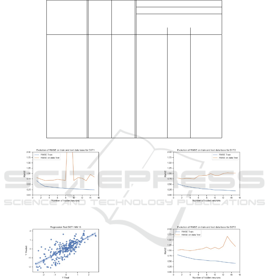
Table 2: T1: RMSE on train and Test datasets, Γ and Hypothesis testing apply to Dryer C.

Conﬁguration Test basis: 254

and Degree of freedom: 253

Number of RMSE RMSE Γ

lower

= 210.84

hidden on on Γ

upper

= 298.95

neurons Train Test Taux Γ Pvalue Result

1 0.67 0.81 378.35 0.00 Reject

2 0.50 0.74 313.46 0.00 Reject

3 0.40 0.67 263.61 0.31 Accept

4 0.38 0.68 270.79 0.21 Accept

5 0.36 0.69 272.73 0.19 Accept

6 0.34 0.73 307.42 0.01 Reject

7 0.32 0.70 287.17 0.07 Accept

8 0.31 0.68 266.84 0.26 Accept

9 0.30 4.95 14 172.39 0.00 Reject

10 0.29 0.67 262.50 0.33 Reject

11 0.28 0.81 376.51 0.00 Reject

12 0.27 0.78 351.20 0.00 Reject

13 0.26 0.66 - - Reference

14 0.25 0.95 523.71 0.00 Reject

15 0.24 0.83 402.57 0.00 Reject

Figure 10: T1 NNC: Evolution of RMSE on train and test

datasets, function of number of hidden neurons.

Figure 11: T1 NNC 13: Regression on test datasets between

Real and Prediction Values.

datasets in function of hidden neurons number. For

similar reasons than for Tube 1, the model ”T2 NN1

5” for dryer 1 Tube 2 is selected. The RMSE values

of this model for the train and test datasets are 0.33

and 0.75 respectively.

Dataset Dryer 2. The same work performed for

dryer 1 Tube 2 (ref:4.1.2.1 ) is applied on Dryer 2

Tube 2. The results are summarized ﬁgure 13 which

presents the evolution of RMSE on train and test

Figure 12: T2 NN1: Evolution of RMSE on train and test

datasets, function of number of hidden neurons.

Figure 13: T2 NN2: Evolution of RMSE on train and test

datasets, function of number of hidden neurons.

datasets in function of hidden neurons number. For

similar reasons than for preceding cases, the model

”T2 NN2 4” for dryer 2 Tube 2 is selected. The RMSE

values of this model for the train and test datasets are

0.65 and 0.99 respectively.

By comparing the accuracy of the models built on

tube 2 datasets (dryers 1 and 2) to those of the tube 1

(dryers 1 and 2) it appears that the modeling of tube 2

is more difﬁcult than that of tube 1.

NCTA 2022 - 14th International Conference on Neural Computation Theory and Applications

386

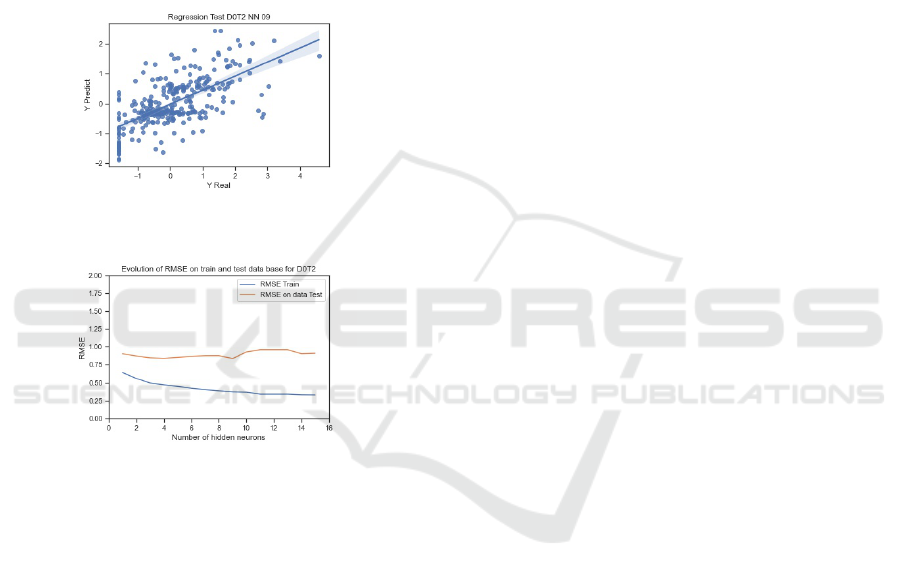
Dataset Dryer Combination. The same work per-

formed for dryer C Tube 1 (ref:4.1.1.3 ) is applied on

Dryer C Tube 2. The optimal structure includes 9 hid-

den neurons (”T2 NNC 9”), with a RMSE on train of

0.37 and a RMSE on test of 0.84. ”T2 NNC 9” can

reach all the points in the test dataset and have not

inconsistent values (regression graphic 14). The per-

formed khi-2 tests accept the conﬁguration 2 on the

test results (RMSE on test 0.87), however the khi-2

test results conﬁrm that other models are statistically

worse on train datasets. That’s why the model ”T2

NNC 9” is selected. The results are summarized ﬁg-

ure 15.

Figure 14: T2 NNC 9: Regression on test datasets between

Real and Prediction Values.

Figure 15: T2 NNC: Evolution of RMSE on train and test

datasets, function of number of hidden neurons.

4.2 Models Comparison

In the previous section (ref 3.1) three models respec-

tively built by using dryer 1, dryer 2 and dryer C

databases, have been selected for tubes 1 and 2. In

this section, these models will be compared in order

to determine if it is possible to use and maintain one

common model rather than one model per dryer.

4.2.1 Tube 1

In a ﬁrst step, the comparison work is performed for

tube 1, beginning with Dryer 1, followed by Dryer 2.

Dryer 1. The goal is to compare the performances

of the best model built by using database dryer 1 ”T1

NN1 3” with the one built by using the combined

database dryer C ”T1 NNC 13”. For this compari-

son, the ”T1 NNC 13” is applied to the test dataset

of Dryer 1, and the RMSE computed is equal to 0.87.

For the Fisher-Snedecor test (F test) used, the RMSE

is used as estimation of the variance of the residuals,

the mean of the residuals is supposed null. The F test,

with parameters explicited in table 3, gives a ratio T

equal to 2.47, above the upper bound of 1.38. The

Pvalue of T is closed to 0.00, so ”T1 NNC 13” gives

results statistically different to those from ”T1 NN1

3”. To conclude for tube 1 of Dryer 1, to use of data

collected on dryer 2 degrades the performances of the

model. This fact may be due to two main causes.

First, the two dryers are actually used into two differ-

ent conditions. Dryer 1 works with fresh wood when

dryer 2 works with recycled wood. So build a spe-

cialized model gives better results than to build a gen-

eralized one. Second, these two dryers, even if they

were identical at the beginning, were able to evolve

differently. However, even if specialized models are

more accurate than combined one, the performances

of combined model remain acceptable.

Dryer 2. The same comparison performed for dryer

1 Tube 1 (ref:4.2.1.1 ) is applied on Dryer 2 Tube 1.

”T1 NNC 13” obtain a RMSE of 2.05.

The F test (Parameter: degree of freedom: 103,

Risk of error: 5%, Lower bound: 0.68 and Upper

bound: 1.47) performed shows that the specialized

model ”T1 NN2 2” gives statistically better results

than the combined one ”T1 NNC 13” (Ratio T of

12.04 and a PValue of 0). However, as for the dryer 1,

the accuracy of the combined model remains accept-

able.

4.2.2 Tube 2

In a second step, the comparison work is performed

for tube 2, in the same process as 4.2.1, starting with

Dryer 1 and then Dryer 2.

Dataset Dryer 1. The comparison between models

”T2 NN1 5” and ”T2 NNC 9” on dryer 1 tube 2 are

the same as Tube 1 of Dryer 1 (4.2.1).1. ”T2 NNC

9” obtains a RMSE of 2.15 on dataset of Tube 2 of

Dryer 1. Parameter of F test are: degree of freedom:

149, risk of error: 5%, lower bound: 0.72 and upper

bound: 1.38. With a Ratio ”T” of 3.86 and a Pvalue

very close to 0.00, the conclusion for tube 2 of Dryer

1 is similar to the one of tube 1 (4.2.1.1), with adding

the effect of intermittent operation due to seasonality.

So the accuracy of model ”T2 NN1 5” is statistically

better than the one of model ”T2 NNC 9” for dryer 1

Tube 2. However, the performances of the combined

model remains acceptable.

A MLP for Dryer Energy Consumption Prediction in Wood Panel Industry

387

Table 3: Tube 1 Dryer 1: Fisher-Snedecor result test between ”T1 NN1 3” and ”T1 NNC 13”.

Freedom degrees: 149 Risk of error: 5% Lower bound: 0.72 Upper bound: 1.38

NN Name and conf. RMSE: test dataset Dryer 1 Ratio ”T” Pvalue Fisher Test

T1 NN1 3 0.35

2.47 0.00 Reject

T1 NNC 13 0.87

Dataset Dryer 2. The same work performed for

dryer 1 Tube 2 (ref:4.2.2.1 ) is applied on Dryer 2

Tube 2. RMSE of ”T2 NNC 9” on this dataset is 2.02.

The parameters are: degree of freedom: 158, risk of

error: 5%, lower bound: 0.73 and upper bound: 1.37.

The results are a ratio of 2.07 and a Pvalue close to

0. One more time, the conclusions are the same. The

specialized model ’T2 NN2 4” is statistically more ac-

curate than the combined one ”T2 NNC 9”. However,

the performances of the combined model remains ac-

ceptable.

5 CONCLUSIONS

In order to model dryers steam consumption be-

haviours, several MLP have been trained on different

datasets. (single or combination dryer). The goal is

to reduce the number of models, because maintain-

ing one model instead of several is easier and cheaper

in changing industrial environment. To conclude this

paper, the construction of a global model represent-

ing the operation of the two dryers is less effective

than the construction of a dedicated model for each

dryer, due to the use of different raw-material (recy-

cled wood vs. fresh wood) and the different modiﬁca-

tions made during their life leading to a drift between

the behaviors of these two dryers. However, even if

dedicated models are more accurate than combina-

tion one, the performances of combined models re-

main acceptable. Also, if a change in the management

policy of the two dryers were to take place (switch

to recycled material or fresh wood on both dryers),

the construction of a global model would make sense.

Moreover, the behaviors of dryers evolve during the

time due to, as example: fouling, wear and tear and

continual improvement actions. To ensure the perfor-

mance and conﬁdence during the time of these model,

it will be interesting to add statistical process control

tools such as control charts to detect when to update

the models (Thomas et al., 2018). In this work, both

dryers were split in two tubes, and tubes was treated

alone. In futur work, it would be interesting to group

together tube from the same dryer, in order to create a

single dataset for each dryer. Then, same work as pre-

sented in this paper could be done, to compare the per-

formances of a specialized neural network trained on

single dryer with a global neural network trained on

combination dryer, which could be easier for mainte-

nance and retraining, and could be used indifferently

for both dryer.

REFERENCES

Azadbakht, M., Aghili, H., Ziaratban, A., and Torshizi,

M. (2016). Application of artiﬁcial neural network

method to exergy and energy analyses of ﬂuidized bed

dryer for potato cubes. Energy.

Buehlmann, U., Ragsdale, C. T., and Gfeller, B. (2000). A

spreadsheet-based decision support system for wood

panel manufacturing. ISPRS Journal of Photogram-

metry and Remote Sensing, 29:21.

Huang, M. and Mujumdar, A. (1993). Use of neural net-

work to predict industrial dryer performance. Dry-

ing Technology: An International Journal, 11(3):525–

541.

Jin, Y., Wong, K. W., Yang, D., Zhang, Z., Wu, W., and Yin,

J. (2021). A neural network model used in continuous

grain dryer control system. Drying Technology: An

International Journal.

Lasi, H., Fettke, P., Kemper, H.-G., Feld, T., and Hoffmann,

M. (2014). Industry 4.0. Business & Information Sys-

tems Engineering, 6(4):239–242.

Martineau, V., Morin, M., Gaudreault, J., Thomas, P., and

Bril El-Haouzi, H. (2021). Neural network architec-

tures and feature extraction for lumber production pre-

diction. In The 34th Canadian Conference on Artiﬁ-

cial Intelligence. Springer.

Nguyen, D. and Widrow, B. (1990). Improving the learning

speed of 2-layer neural networks by choosing initial

values of the adaptive weights. 1990 IJCNN Interna-

tional Joint Conference on Neural Networks, 3:21–26.

Sapna, S. (2012). Backpropagation learning algorithm

based on levenberg marquardt algorithm. Computer

Science & Information Technology ( CS & IT ), pages

393–398.

Thomas, P., El Haouzi, H. B., Suhner, M.-C., Thomas, A.,

Zimmermann, E., and Noyel, M. (2018). Using a clas-

siﬁer ensemble for proactive quality monitoring and

control: The impact of the choice of classiﬁers types,

selection criterion, and fusion process. Computers in

Industry, 99:193–204.

Thomas, P. and Thomas, A. (2011). Multilayer percep-

tron for simulation models reduction: Application to

a sawmill workshop. Engineering Applications of Ar-

tiﬁcial Intelligence, 24(4):646–657.

NCTA 2022 - 14th International Conference on Neural Computation Theory and Applications

388