Machine Learning based Predictive Maintenance in Manufacturing

Industry

Nadeem Iftikhar

, Yi-Chen Lin and Finn Ebertsen Nordbjerg

Department of Computer Science, University College of Northern Denmark, Aalborg 9200, Denmark

Keywords:

Predictive Maintenance, Condition Based Maintenance, Machine Learning, Industry 4.0, Time Series.

Abstract:

Predictive maintenance normally uses machine learning to learn from existing data to ﬁnd patterns that can

assist in predicting equipment failures in advance. Predictive maintenance maximizes equipment’s lifespan by

monitoring its condition thus reducing unplanned downtime and repair cost while increasing efﬁciency and

overall productive capacity. This paper ﬁrst presents the machine learning based methods to predict unplanned

failures before they occur. Afterwards, to confront the everlasting downtime problem, it discusses anomaly

detection in greater detail. It also explains the selection criteria of these methods. In addition, the techniques

presented in this paper have been tested by using well-known data-sets with promising results.

1 INTRODUCTION

Nowadays, machines are not only critical to manufac-

turing industry but to every industry. Corrective main-

tenance or reactive maintenance is usually performed

to reinstate machines to acceptable functioning condi-

tions after a break down or failure. Corrective main-

tenance can lead to higher maintenance costs and un-

planned downtime. Predictive maintenance (PdM) on

the other hand keeps the machinery in healthy con-

dition by accurately predicting when the failure or

break down might occur and have corrective mea-

sures in place. Thus reducing unplanned downtime

and increasing equipment’s lifespan. Some examples

of PdM with respect to ball bearing are: to detect

bearing life (due to wear and tear) before it fails; to

ﬁnd out whether a bearing needs lubrication or not;

to raise an alarm when lubricant is contaminated and

so on. PdM is usually based on statistical analyses

and machine learning algorithms in order to estimate

anomalous behavior, remaining useful life (RUL) and

time-to-failure (TTF).

Machine learning (ML) based PdM falls under

two types of learning, supervised and unsupervised.

Supervised learning is based on building predictive

models or making forecasts. Supervised learning re-

quires historical data of both input and output, which

means that there must be labelled data available. Su-

pervised learning algorithms mainly consist of regres-

https://orcid.org/0000-0003-4872-8546

sion and classiﬁcation. Regression based algorithms

take input data and produce continuous output value,

for example the amount of time until the machine or

one of its components hit failure condition or remain-

ing useful life (RUL) of a component. Further, classi-

ﬁcation based algorithms take input data and produce

discrete output, such as machine or one of its compo-

nents failure is inevitable.

On the other hand, for unsupervised learning there

is no labeled data or output available and there is also

no information about how machine failures look like

in the data. Unsupervised learning does not perform

forecasts, however it can be used to identify anoma-

lous behavior. Anomalous behavior can be caused

by some kind of rare events or observations. Fur-

thermore, it provides additional insight into the inher-

ent structure of the data and helps to discover hidden

patterns and correlations in the data. It can also be

used to divide data into clusters based on their resem-

blances or dissimilarities.

To summarize, the main contributions in this pa-

per are as follow:

• Applying a methodological approach for PdM us-

ing ML.

• Presenting a set of criteria for selecting a speciﬁc

PdM approach.

• Focusing on the taxonomy of unsupervised

anomaly detection techniques.

The paper is structured as follows. Section 2

presents the related work. Section 3 describes the

Iftikhar, N., Lin, Y. and Nordbjerg, F.

Machine Learning based Predictive Maintenance in Manufacturing Industry.

DOI: 10.5220/0011537300003329

In Proceedings of the 3rd International Conference on Innovative Intelligent Industrial Production and Logistics (IN4PL 2022), pages 85-93

ISBN: 978-989-758-612-5; ISSN: 2184-9285

methodological approach to accomplish a ML-based

project. Section 4 explains the PdM techniques. Sec-

tion 5 discusses the applications of ML methods for

PdM. Section 6 concludes the paper and points out

the future research directions.

2 RELATED WORK

This section mainly concentrates on the previous

work done in relation to ML based PdM for smart

manufacturing. A state-of-the-art review of ML tech-

niques for PdM is presented by (Carvalho et al.,

2019). An end-to-end ML based predictive main-

tenance approach for manufacturing is provided by

(Ayvaz and Alpay, 2021). The proposed system is

scalable and effective for high-dimensional stream-

ing data. The system is also implemented in a real

manufacturing factory with success. Further, (Ouadah

et al., 2022) described the process of selecting the

most suitable supervised ML methods for PdM. Sim-

ilarly, (Hosamo et al., 2022) used supervised ML

techniques to forecast the equipment’s state in order

to plan maintenance in advance. In addition, vari-

ous supervised ML algorithms such as, logistic re-

gression, neural networks, support vector machines,

decision trees and k-nearest neighbors were applied

to predict costly production line disruptions (Iftikhar

et al., 2019). The accuracy of the proposed ML mod-

els were tested on a real-world data set with promis-

ing results. Furthermore, (Garan et al., 2022) men-

tioned the beneﬁts of a data-enteric ML methodology

for predicting RUL. A supervised learning based pre-

dictive model to predict failure within a ﬁxed time

period (at least 4 hours in advance) is presented by

(Herrero and Zorrilla, 2022). PdM for aircraft engines

has been studied by (Azyus and Wijaya, 2022) using

both classiﬁcation and regression techniques. Like-

wise, the work by (Schwendemann et al., 2021) pro-

vided an overview of the most important approaches

for bearing-fault analysis, ﬁrst based on classiﬁcation

to detect the unhealthy condition, position and sever-

ity of the fault, later based on regression to predict the

RUL.

Moreover, a ML based PdM system for manufac-

turing industry is developed by (Arena et al., 2022)

to estimate the RUL based on ensemble models. A

feature selection strategy for unsupervised learning

is presented by (Yang et al., 2011). This work sug-

gested that fewer features could help to maximize the

performance of unsupervised learning models. (Kre-

mer et al., 2021) applied a deep learning method

for anomaly detection. Additionally, ensemble based

prediction models are implemented using supervised

and unsupervised learning (Rousopoulou et al., 2020)

and (Iftikhar et al., 2020), respectively. Finally,

a structured and comprehensive survey provided an

overview of the anomaly detection techniques (Chan-

dola et al., 2009). The work presented in this pa-

per considers a number of the recommendations pre-

sented in (Chandola et al., 2009).

The focus of the previous works is on various as-

pects and recent advancements of PdM using ML.

Most of these works focus on selecting ML models

for PdM and comparing their performance. On the

other hand, the work presented in this paper empha-

sises on the practical issues in relation to PdM. In ad-

dition, it covers most of the scenarios with respect to

PdM based on both labeled and unlabeled data.

3 METHODOLOGY

The development methodology used in this paper

is based on the data science workﬂow: CRoss In-

dustry Standard Process for Data Mining (CRISP-

DM)

. CRISP-DM is a robust, proven and generally

used methodology for planning, organizing and im-

plementing ML projects. CRISP-DM consists of the

following six phases: business understanding, data

understanding, data preparation, modeling, evalua-

tion, and deployment.

• Business understanding: One of the major ﬂaws

with ML-based projects in PdM is to start with

data gathering and model building rather than

business understanding. Different areas of interest

have different concerns and anticipations. Firstly,

business objectives/goals should be deﬁned. Fol-

lowed by use cases that accomplish the deﬁned

goals along with the tools/technologies that are re-

quired to full-ﬁll these objectives.

• Data understanding: Once the business cases are

developed, the next step is to collect and under-

stand data. At this stage there are two common

scenarios, either the data can be/has been col-

lected by using existing sensors or there is a need

to set up new/additional sensors to collect data

that is required to fulﬁll the requirements of the

use case(s). In the ﬁrst scenario, a ML model

is selected in order to best suit the data at hand,

whereas in the second scenario right data needs to

be collected based on a pre-planned ML model.

The most important question to answer at this

stage is “can already/potentially available data be

used to achieve the deﬁned business goals?”. To

gain insight into the acquired data, exploratory

https://thinkinsights.net/digital/crisp-dm

IN4PL 2022 - 3rd International Conference on Innovative Intelligent Industrial Production and Logistics

data analysis (EDA) is performed. EDA is helpful

in order to understand the structure of the data and

to see if there is further cleansing required, or if

there is a need to acquire more data. By combing

business and data understanding, hypotheses are

also being made during this phase in order to suc-

cessfully develop a ML-based project for PdM.

• Data preparation: Data at this phase is processed

to prepare for predictive modeling. Several tech-

niques are used here, for instance data cleansing

and feature engineering. In order to build a ML

model for PdM, both historical and static data is

normally required. Historical data includes main-

tenance and failure history of the equipment. It

also includes information about events leading to

failure process. Where as, static data contains me-

chanical properties of the equipment, usage of the

equipment, operating conditions and so on.

• Modeling: In this phase, several different algo-

rithms/models are applied to a broad range of use

cases. In order to perform predictive maintenance,

more modelling options are available in super-

vised as compared to unsupervised learning. For

instance, to estimate RUL, similarity model could

be used if run-to-failure data is available. Similar-

ity model is able to detect patterns that represent

both normal operating condition as well as equip-

ment failures. Opposite to the similarity model is

the anomaly model that is able to detect patterns

that do not match with normal operating condi-

tions. Further, survival model as probability dis-

tribution could be used if lifetime data is avail-

able that indicates how long it took for similar ma-

chines to reach failure. Furthermore, degradation

model could be used (based on a condition indica-

tor/threshold that detects failure) if there is no or

some life-history and/or failure data is available.

As different models can be used, it is important to

discuss if the outcome meets the business objec-

tives. If data is not applicable for meeting the ex-

pectations, other solutions should be considered,

like ﬁnding suitable data or adjusting the goal(s).

• Evaluation: To effectively evaluate the perfor-

mance of the selected models, different evalu-

ating techniques are used to ﬁnd the most suit-

able model. For example, classic regression

model could be evaluated using R-Squared, mean

absolute error (MAE), root mean squared error

(RMSE) and so on. However, in the case of RUL,

the error could be the difference between pre-

dicted life and actual life. Similarly, confusion

matrix and F1-score are common techniques to

evaluate a classiﬁcation model. Evaluating an un-

supervised model is not as straightforward as su-

pervised ones since there is no labeled data avail-

able. Though, if data is labeled by domain ex-

perts ﬁrst or data has only normal behaviour, in

that case F1-score, precision, recall and accuracy

could be used to evaluate the model, otherwise

the results should be veriﬁed by the domain ex-

perts. If the results still need improvements or

adjustments, revisiting the business and data un-

derstanding phases is advisable.

• Deployment: After deploying the best model and

in order to get better predictions, it is necessary to

constantly monitor and reﬁne the model. Hence,

the CRISP-DM methodology runs in a circle to

continuously improve the model.

4 PREDICTIVE MAINTENANCE

In general, the selection of ML methods for PdM is

based on the underlying maintenance policy, however

this selection can be categorized into the following

three approaches. If the goal is to predict how much

time is left before the next failure (RUL) or to pre-

dict whether there is a possibility of failure in a ﬁxed

time frame, in both these case supervised learning

can be used. Further, to detect anomalous behav-

ior on that occasion unsupervised learning or semi-

supervised learning can be utilized, however there is

of course a little more to that perception. Hence, in

the following three sections, the adoption process of

these three methods is discussed in detail.

4.1 Supervised Machine Learning

Methods

Knowing what to predict will assist in deciding which

ML method to use. Normally, classiﬁcation based

methods predicts sudden equipment failure using less

data with greater precision, where as regression based

methods provides more information about the failure

and when it will happen though it needs more data.

4.1.1 Regression based Models

Regression based models are commonly used to pre-

dict the RUL (Fig. 1) of an equipment on the assump-

tion that following requirements are satisﬁed:

• Data should be labeled.

• Availability of both historical data (machine break

downs and maintenance history) as well as static

data (machine speciﬁcations).

• Data should contain both normal and failure

events.

Machine Learning based Predictive Maintenance in Manufacturing Industry

• Each model will focus on only one type of failure.

• The failure process is gradual.

In general, the regression-based RUL estimating

models can be divided into three categories: simi-

larity, degradation and survival (Fig. 1). Similarity-

based models are used when there is run-to-failure

data available from similar machines in other words

complete histories from acceptable conditions to fail-

ure conditions are available. Further, survival mod-

els are used when there is only failure data available

from the similar machines (there is no complete histo-

ries though only failure conditions are known). Fur-

thermore, degradation model are used when there is

no failure data available, however there would be a

threshold value that could triggers a failure condition

when crossed or a known threshold value of a condi-

tion indicator that detects failure conditions. All these

three above mentioned models can be seen in Fig. 1.

Time

Acceptable Condition

Minimal Acceptable Condition

(Condition Indicator)

Failure Condition

RUL

Similarity Model

Degradation Model

Survival Model

Figure 1: Remaining Useful Life of an equipment.

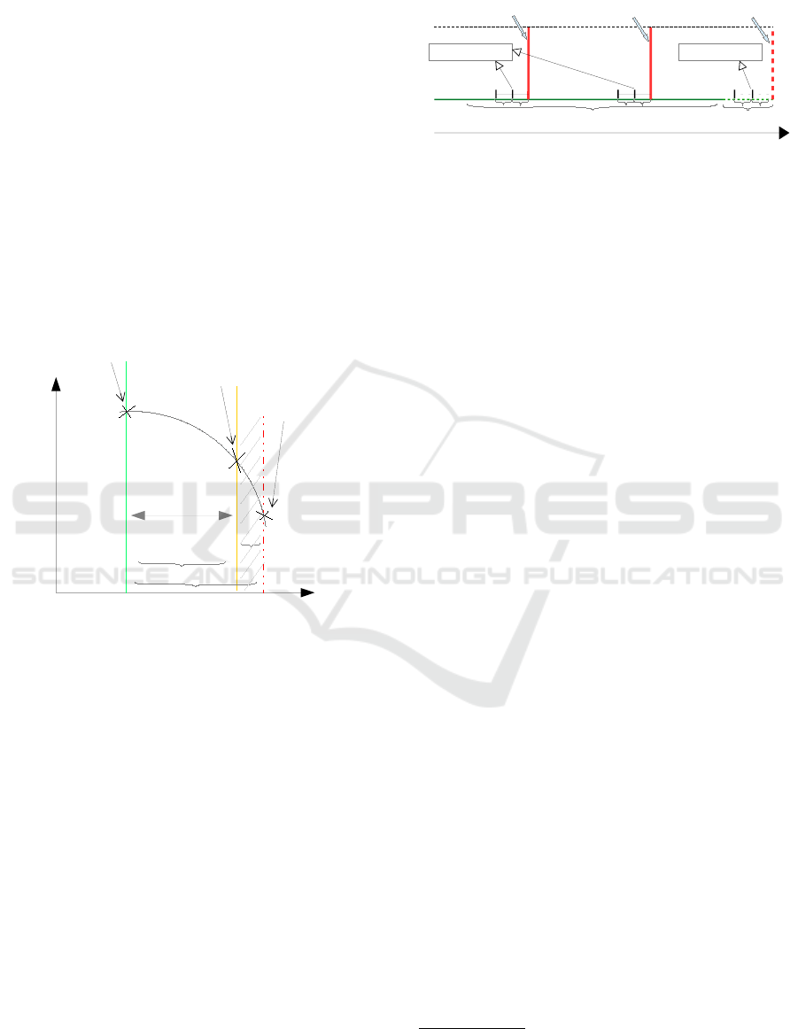
4.1.2 Classiﬁcation based Models

Classiﬁcation based models are used to predict “if a

sudden failure is imminent” (Fig. 2). These mod-

els are divided into two categories, binary and multi-

class. Binary models can predict categorical class la-

bels “failure or not” as well as failure type (i.e. if

the information about failure type(s) is available in

the data-set). Further, classiﬁcation based models can

also predict “will an equipment fail in a given pe-

riod of time window”, such as in next 5 hours or [1

- 25] cycles window (w1). Where, w1 is a prede-

ﬁned time/cycles related parameter, which can be in-

serted as an extra column in the training set during

data preprocessing. Normally, the length of w1 is de-

cided by domain experts based on how far ahead of

time the failure-alarm should trigger before the actual

failure. Similarly, multi-class models can predict “in

which period range or cycles window will component

X fail due to fault Y”. For example, periods could be

in range of [1 - 5] hours window w1, [6 - 10] hours

window w2 , [11 - 15] hours window w3 and so on.

Equipment FailedEquipment Failed

Normal

NormalNormal

Equipment Failure

is Imminent

Historical Data Recent Data

Time/Number of Cycles

Historical time before

failure window(s)

w1w1w2 w2 w1w2

Predicted time before

failure window(s)

Figure 2: Binary classiﬁcation of equipment failure.

The preconditions for choosing the classiﬁcation

based models are almost same as the regression based

models, except that multi-class classiﬁcation mod-

els could focus on multiple types of failures and

most importantly the failure process should be sud-

den (Fig. 2).

4.2 Unsupervised Machine Learning

Methods

In most cases, labeled data is not easily available,

however it is still possible to implement a PdM strat-

egy for unlabelled data (or data that does not contain

failure events) using unsupervised learning. Unsuper-

vised learning is capable of anomaly detection, clus-

tering, association and dimensionality reduction. In

this paper, the main emphasis is on detecting anoma-

lous behavior, hence the rest of the methods are

not explored further. Even though, anomalies occur

rarely, however they cause abrupt machine failures.

In general, anomaly detection focuses on detecting

abnormal patterns/behaviours that diverge from the

rest of the data/group. Further, anomalies detection

can also be speciﬁed as outlier detection and nov-

elty detection. Novelties are new observations that

are not similar to the existing data. Where as, out-

liers are unexpected observations due to extraordinary

situations. Both, novelty and outlier detection uses

slightly different detection approaches. In novelty de-

tection, the training set only contains “normal” data-

points and the testing set contains both “normal” and

“faulty” data-points. Where as, novelty detection is

more a semi-supervised than an unsupervised learn-

ing method for the reason that it is based on one-class

classiﬁcation. On the other hand, in outlier detection,

the training and testing sets both contain “normal” as

well as “faulty” data-points.

One of the most important goals of this paper

is to explore different anomaly types, concepts and

anomaly detection techniques

. To start with, there

https://iwringer.wordpress.com/2015/11/17/anomaly-

detection-concepts-and-techniques

IN4PL 2022 - 3rd International Conference on Innovative Intelligent Industrial Production and Logistics

No Training Data

Anomaly

Point Anomaly Collective Anomaly

Contextual Anomaly

Training Data

Statistical

Methods

Median,

Median Absolute

Deviation and

Robust Z-Score

Univariate Multivariate

Parametric

Nonparametric NonParametric

Parametric

Decision

Tree Methods

Isolation Forest

Covariance

Methods

Distance & Density,

Kernel and

Decision Tree Methods

Local Outlier Factor

One-class SVM

Isolation Forest

No Training Data Training Data

MultivariateUnivariate

Stochastic

Methods

Markov Chain

Ordered Unordered

Clustestring

Methods

K-Means /

K-Medians

Mix of Clustering

& Stochastic

Methods

K-Means /

K-Medians

Markov Chain

Parametric

Nonparametric

Covariance

Methods

Elliptic

Envelope

Distance &

Density

Methods

Local Outlier

Factor

Clustering

Methods

K-Means /

K-Medians

Statistical

Methods

Median,

Median Absolute

Deviation and

Robust Z-Score

Elliptic

Envelope

Figure 3: Anomaly types and unsupervised learning based detection techniques.

are three types of anomalies: point anomalies; col-

lective anomalies; and contextual anomalies (Fig. 3).

Point anomaly deals with a single data-point that

is out of the ordinary with respect to rest of the

data, such as a single electricity consumption value

that ascends from the baseline. Where as, collective

anomaly deals with a collection of similar data-points,

which could be considered as anomalous in relation to

the rest of the data, for example a successive 5 hour

period of high electricity consumption. Moreover,

contextual anomaly have to do with data-points con-

sidered anomalous with respect to other data-points

within the same context, for instance low electricity

consumption at noon during week days (i.e. every

member of a family could be at work or at school).

Further, as shown in (Fig. 3), it is possible to de-

tect anomalous behaviour with or without training

data. Both point and collective anomaly detection

techniques could be univariate or multivariate. Uni-

variate means that there is only one time-dependent

variable present in order to detect anomalous behav-

ior, such as temperature. Multivariate indicates that

there are multiple time-dependent variables present to

detect anomalous behaviour based on a single model,

for example temperature, humidity, CO2 and noise.

Furthermore, training data based anomaly detection

techniques could be parametric or nonparametric.

Parametric means that the underlined distribution is

known and/or data (∼ 50%) is normally distributed

and nonparametric means that either no information

about the data distribution is available and/or data

could be skewed or fat-tailed. Moreover, no train-

ing data based collective multivariate anomalies could

be either ordered or unordered. Ordered anomaly

detection represents that events could be in unex-

pected order/pattern, such as a segment of sequences

from 3 sensors (current, pressure and temperature) in

the same time interval gained a systematic or sud-

den change in the pattern from the previous patterns.

Unordered anomaly detection represents unexpected

value combinations of a set of unordered variables, for

example if there are 2 sensors attached to a bearing,

generating 2 different signals: bearing vibration and

bearing temperature. The readings of those signals

individually may not tell much on bearing-level risks,

however when combined together, these signals can

represent the health of the bearing. The signals may

be acquired at every n minutes and a health-index is

calculated, so if the health-index represents an unex-

pected pattern from the previous patterns then it could

be triggered as an anomalous behaviour. Finally, as

seen in Fig. 3, depending on the type of anomaly a

particular statistical, stochastic or machine learning

based model could be used.

5 PREDICTIVE MAINTENANCE

APPLICATIONS

To forecast future machine deterioration/failure based

on sensor values such as, vibrations, temperature,

pressure and so on, supervised learning can be used

either to estimate what is the RUL or to forecast the

upcoming failure (TTF). In addition, unsupervised

learning can be used to ﬁnd anomalous behavior in

an equipment.

Machine Learning based Predictive Maintenance in Manufacturing Industry

5.1 Estimating Remaining Useful Life

(RUL) with Degradation Model

In order to estimate the RUL, NASA’s lithium-ion

battery or Li-ion battery prognostics data-set is used

(Song, 2019). Lithium-ion batteries are quite popular

these days as their applications range from portable

electronics to electric vehicles. These batteries are

rechargeable, however they lose capacity gradually

due to frequent charging/recharging (charge cycles).

In order to avert unplanned downtime, sudden capac-

ity loss should be avoided by predicting the RUL of

these batteries. To predict RUL several degradation-

based regression models are used in this paper. Ac-

cording to (Sahaand and Goebel, 2007), the end of

life (EoL) of Li-ion battery is considered when the

capacity drops to 70% of the initial value. Thus, the

EoL threshold can be taken as a condition indicator to

calculate remaining useful cycles as in Fig. 4.

Battery Capacity

End-of-life Threshold

Number of Cycles

0 25 50 75 100 125 150 175

1.8

1.7

1.6

1.5

1.4

1.3

Figure 4: Capacity vs cycle number.

From the NASA’s data-set battery B5 is chosen to

estimate the RUL. There are three operations in the

original data-set: charge, discharge and impedance.

Based on (Khumpromand and Yodo, 2019) sugges-

tion, discharge operation is used to estimate the RUL.

The discharge consists of 164 cycles and 11,345 data

points. Further, the data-set contains 10 features with

no missing or duplicated values. As the data-set is

high-dimensional, feature importance ranking is done

by random forest feature importance

to identify neg-

ligible features in order to improve the efﬁciency

and effectiveness of the predictive model. The result

shows that cycle is the only important contributor to

capacity among all features. Cycle and capacity have

high negative correlations. In other words, increasing

the number of cycles decreases the capacity. The split

ratio used between training and testing set is 80/20.

Firstly, independent/input X includes all the features

https://machinelearningmastery.com/calculate-

feature-importance-with-python

expect capacity which is deﬁned as continuous depen-

dent/output Y. Afterwards, based on the result of fea-

ture importance ranking, independent/input X that in-

cludes only cycles is modeled in order to compare the

performance.

Table 1: Evaluation of regression based models for RUL (*

dimension reduction).

Model RMSE R2-score Error cycle

SVR 0.048 -4.028755379916393 -2

SVR* 0.041 -2.4280651482293845 -2

LassoLarsCV 0.050 -4.48447130580669 0

SGDRegressor* 0.017 0.393702606072853 2

Due to the high-dimensional nature of the NASA

data-set, support vector regression (SVR) is chosen as

the main regression model. SVR can solve linear and

non-linear problems and has the ability to automati-

cally regularized the features (by ignoring insigniﬁ-

cant features), thus preventing over-ﬁtting. In addi-

tion to SVR, the tree-based pipeline optimization tool

(TPOT) - AutoML

is also used in this paper. AutoML

is used to automate the selection, comparison and pa-

rameter tuning process of the ML models.

Table 1, shows the performance comparison of

SVR and the models selected by AutoML. In Ta-

ble 1, remaining cycles error (error cycle) is calcu-

lated by subtracting the predicted number of cycles

from the actual number of cycles. root mean square

error (RMSE) and R2-score of SVR and SVR* (with

reduced dimensional data) is almost same, however

the computation time of SVR* is 99% lower than

SVR (from 3 minutes to 0.4 second). Similarly, the

computation time of ﬁnding the best model by Au-

toML is 99% lower than manually ﬁnding the best

ML model (from 60 minutes to 60 seconds). R2-score

measures how well the models ﬁts and usually it has

a range between 0 and 1.

To summarise, SGDRegressor* (with reduced di-

mensional data) gives the best RMSE and R2-score

among all the models. Additionally, the visualized

results of RUL predictions are presented in Figure 5.

Generally, all the models perform well, SGDRegres-

sor* performed the best (Figure 5(d)). Figure 5(a) is

the SVR result of RUL prediction. As there are lots

of features within the data-set, the predicted line is

not smooth. Figure 5(b) is the result of SVR* ﬁtted

with dimensional reduced data. Further, Figure 5(c) is

the LassoLarsCV result of RUL. LassoLarsCV tends

to over-ﬁt as actual and predicted capacity values are

overlapped.

http://automl.info/tpot

IN4PL 2022 - 3rd International Conference on Innovative Intelligent Industrial Production and Logistics

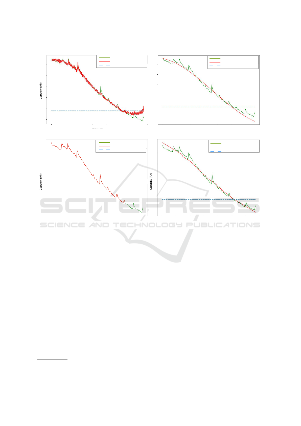
Support Vector Regression (SVR)

LASSO-LARS Cross-Validation (LassoLarsCV)

Stochastic Gradient Descent Regressor (SGDRegressor*)

0 25 50 75 100 125 150 175

Support Vector Regression (SVR*)

Actual Capacity

Predicted Capacity

End-of-life Threshold

Actual Capacity

Predicted Capacity

End-of-life Threshold

Actual Capacity

Predicted Capacity

End-of-life Threshold

Actual Capacity

Predicted Capacity

End-of-life Threshold

1.8

1.7

1.6

1.5

1.4

1.3

1.8

1.7

1.6

1.5

1.4

1.3

1.8

1.7

1.6

1.5

1.4

1.3

1.8

1.7

1.6

1.5

1.4

1.3

(

)

Number of Cycles

(d)

Number of Cycles

(c)

Number of Cycles

(a)

Number of Cycles

(b)

Figure 5: RUL Prediction.

5.2 Time-To-Failure (TTF) Detection

To predict TTF, bearing data-set from Case Western

Reserve University (CWRU)

is used. In general, ac-

cording to (Kamat et al., 2021), bearing failure causes

30-40% of machine failures. There are several rea-

sons that cause bearing failures, for example over-

loading, faulty installation, improper lubrication and

so on. A sudden bearing failure can cost tens of thou-

sands of dollars per hour when it stops production.

Hence, it is critical to predict “whether a component

has high chance of failure”. CWRU data-set contains

vibration information of both normal and faulty bear-

ings. The data-set consists of 250,000, data-points out

of which 50% are normal and 50% are failures. The

data-set holds no missing values, however it has 6941

duplicates values (which have been removed). The

data-set is made up of three features. To avert un-

planned downtime, sudden bearing failure should be

https://engineering.case.edu/bearingdatacenter

avoided by predicting the TTF. To predict TTF vari-

ous classiﬁcation models are used in this paper. Fur-

ther, in the selected data-set “label=0” is treated as

normal baseline data and “label=1” is treated as fail-

ure data. The data is divided into training set and test-

ing set with 80/20 split. Independent/input X includes

all the features (two in this case) expect fault class

which is deﬁned as continuous dependent/output Y.

The classiﬁcation models are normally evaluated

based on F1-score. It ranges from 0 to 1. F1-score

associates the precision and recall of a classiﬁer with

their numerical average. While, accuracy shows how

many times the model was correct overall. Further-

more, it can be seen in Table 2 that most of the classi-

ﬁers models performed well with respect to F1-score,

besides logistic regression and LinearSVC.

5.3 Anomaly Detection

To estimate anomalous behavior, CWRU bearing

data-set is used. CWRU data-set is the same data-

Machine Learning based Predictive Maintenance in Manufacturing Industry

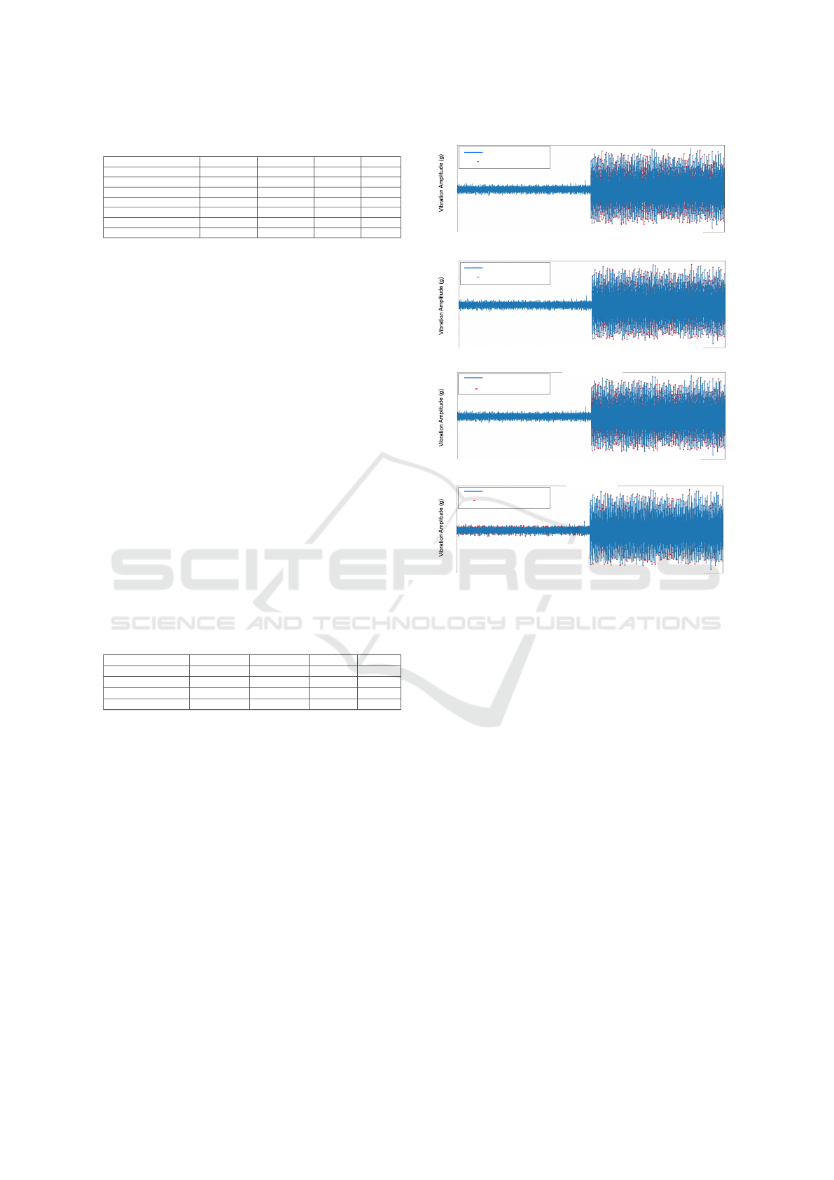
Table 2: Evaluation of classiﬁcation models for TTF.

Model Accuracy (%) Precision (%) Recall (%) F1-score

Logistic Regression 46.40 48.70 90.77 0.63

K-Nearest Neighbors 84.89 89.15 80.21 0.84

LinearSVC 51.12 51.12 100.00 0.68

RBFSVC 86.46 95.48 77.16 0.85

GaussianNB 86.05 94.23 77.46 0.85

Decision Tree 87.51 88.08 87.39 0.88

Random Forest Classiﬁer 84.35 88.28 80.00 0.84

set used in section 5.2 though the target class labels

have been removed for the purpose of applying un-

supervised learning. Thus, description of the data-

set is omitted here. Further, in this paper both nov-

elty detection and outlier detection are used to detect

anomalies. Outlier detection is based on unsupervised

learning, where as novelty detection is based on semi-

supervised learning. In case of novelty detection,

the training set consists of only normal data-points

though the testing set contains both anomalous and

normal data-points. In the event of outlier detection,

the training and testing set both contain anomalous

and normal data-points. Furthermore, covariance-

based elliptic envelope (EE), tree-based isolation for-

est (IF) and density-based (LOF) are used for outliers

detection. In addition, kernal-based one-class support

vector machine (SVM) is used for novelty detection.

The split ratio between training and testing set for

EE, IF and LOF is 80/20 (40/20 in case of one-class

SVM). Moreover, EE is parametric, where as one-

class SVM, IF and LOF are nonparametric. All these

models can be used for univariate as well as multivari-

ate data.

Table 3: Evaluation of anomaly detection models.

Model Accuracy(%) Precision(%) Recall(%) F1-score

One-class SVM 63.00 57.47 100.00 0.73

Elliptic Envelope 60.32 55.75 100.00 0.72

Isolation Forest 67.42 60.54 100.00 0.75

Local Outlier Factor 52.38 51.32 92.38 0.66

The evaluation of the anomaly detection models

is presented in Table 3 and their performance is vi-

sualized in Figure 6. Since, testing set contains both

normal and anomalous data-points. Hence, it can be

observed in Figure 6 that ﬁrst 25,000 data-points are

normal and last 25,000 data-points are anomalous.

The visualization results demonstrate that all the mod-

els did a reasonable job in identifying the anomalies,

which can also be conﬁrmed from F1-score in Table 3.

6 CONCLUSIONS

In manufacturing industry, production line break-

downs cost ∼ 50,000 US$ per hour, worldwide. Fur-

ther, maximum availability of machines and systems

must be preserved in order to meet the demands of

Elliptic Envelope (EE)

Isolation Forest (IF)

(b)

(c)

Vibration Signals

Predicted Anomalies

Vibration Signals

Predicted Anomalies

Vibration Signals

Predicted Anomalies

1.5

1.0

0.5

0.0

-0.5

-1.0

-1.5

1.5

1.0

0.5

0.0

-0.5

-1.0

-1.5

0 10000 20000 30000 40000

Data-points

Vibration Signals

Predicted Anomalies

1.5

1.0

0.5

0.0

-0.5

-1.0

-1.5

0 10000 20000 30000 40000

Data-points

(a)

Data-points

(d)

One-class Support Vector Machine (SVM)

Local Outlier Factor (LOF)

1.5

1.0

0.5

0.0

-0.5

-1.0

-1.5

Vibration Signals

Predicted Anomalies

Figure 6: Visualization of anomaly detection results.

Industry 4.0. This paper applied anomaly detection

and prediction based models to identify abnormal be-

haviours and to forecast equipment failures. By spot-

ting unusual behaviour that differs signiﬁcantly from

what has been observed before can greatly help the

manufacturing industry to reduce unplanned down-

time. The experiments demonstrated that PdM along

with suggested ML methods gives promising results.

In future, deep learning should be investigated for

PdM. In addition, scalability of the presented PdM

techniques could also be explored.

REFERENCES

Arena, S., Florian, E., Zennaro, I., Orr

u, P. F., and Sgar-

bossa, F. (2022). A novel decision support system

for managing predictive maintenance strategies based

on machine learning approaches. Safety Science,

146:105529.

Ayvaz, S. and Alpay, K. (2021). Predictive maintenance

system for production lines in manufacturing: A ma-

chine learning approach using iot data in real-time.

Expert Systems with Applications, 173:114598.

Azyus, A. F. and Wijaya, S. K. (2022). Determining the

IN4PL 2022 - 3rd International Conference on Innovative Intelligent Industrial Production and Logistics

method of predictive maintenance for aircraft engine

using machine learning. Journal of Computer Science

and Technology Studies, 4(1):1–6.

Carvalho, T. P., Soares, F. A., Vita, R., Francisco, R. D. P.,

Basto, J. P., and Alcal

a, S. G. (2019). A systematic

literature review of machine learning methods applied

to predictive maintenance. Computers & Industrial

Engineering, 137:106024.

Chandola, V., Banerjee, A., and Kumar, V. (2009).

Anomaly detection: A survey. ACM Computing Sur-

veys, 41(3):1–58.

Garan, M., Tidriri, K., and Kovalenko, I. (2022). A data-

centric machine learning methodology: Application

on predictive maintenance of wind turbines. Energies,

15(3):826.

Herrero, R. D. and Zorrilla, M. (2022). An i4. 0 data inten-

sive platform suitable for the deployment of machine

learning models: a predictive maintenance service

case study. Procedia Computer Science, 200:1014–

1023.

Hosamo, H. H., Svennevig, P. R., Svidt, K., Han, D., and

Nielsen, H. K. (2022). A data-centric machine learn-

ing methodology: Application on predictive main-

tenance of wind turbines. Energy and Buildings,

261:111988.

Iftikhar, N., Baattrup-Andersen, T., Nordbjerg, F. E., and

Jeppesen, K. (2020). Outlier detection in sensor data

using ensemble learning. Procedia Computer Science,

176:1160–1169.

Iftikhar, N., Nordbjerg, F. E., Baattrup-Andersen, T., and

Jeppesen, K. (2019). Industry 4.0: sensor data analy-

sis using machine learning. In International Confer-

ence on Data Management Technologies and Applica-

tion, pages 37–58. Springer.

Kamat, P., Marni, P., Cardoz, L., Irani, A., Gajula, A., Saha,

A., Kumar, S., and Sugandhi, R. (2021). Bearing fault

detection using comparative analysis of random for-

est, ann, and autoencoder methods. In Communication

and Intelligent Systems, pages 157–171. Springer.

Khumpromand, P. and Yodo, N. (2019). A data-driven

predictive prognostic model for lithium-ion batter-

ies based on a deep learning algorithm. Energies,

12(4):660.

Kremer, O. S., Cunha, M. A., and Silva, P. H. (2021). Imple-

mentation of a predictive maintenance system using

unsupervised anomaly detection. Sim

osio Brasileiro

de Automac¸

ao Inteligente-SBAI, 1(1).

Ouadah, A., Zemmouchi-Ghomari, L., and Salhi, N. (2022).

Selecting an appropriate supervised machine learning

algorithm for predictive maintenance. The Interna-

tional Journal of Advanced Manufacturing Technol-

ogy, 119(7):4277–4301.

Rousopoulou, V., Nizamis, A., Vafeiadis, T., Ioannidis, D.,

and Tzovaras, D. (2020). Predictive maintenance for

injection molding machines enabled by cognitive an-

alytics for industry 4.0. Frontiers in Artiﬁcial Intelli-

gence, 3:578152.

Sahaand, B. and Goebel, K. (2007). Battery data set,

nasa ames prognostics data repository. Available on-

line at: http://ti.arc.nasa.gov/project/prognostic-data-

repository.

Schwendemann, S., Amjad, Z., and Sikora, A. (2021).

A survey of machine-learning techniques for condi-

tion monitoring and predictive maintenance of bear-

ings in grinding machines. Computers in Industry,

125:103380.

Song, S. (2019). Nasa. Available online at:

https://dx.doi.org/10.21227/fhxc-ga72.

Yang, Y., Liao, Y., Meng, G., and Lee, J. (2011). A hy-

brid feature selection scheme for unsupervised learn-

ing and its application in bearing fault diagnosis. Ex-

pert Systems with Applications, 38(9):11311–11320.

Machine Learning based Predictive Maintenance in Manufacturing Industry