Universally Hard Hamiltonian Cycle Problem Instances

Joeri Sleegers

1 a

, Sarah L. Thomson

2 b

and Daan van Den Berg

3 c

Mice & Man Software and A.I. Development, Amsterdam, The Netherlands

Department of Computing Science & Mathematics, University of Stirling, U.K.

Department of Computer Science, Vrije Universiteit Amsterdam, The Netherlands

Keywords:

Exact Algorithms, Instance Hardness, Evolutionary Algorithms, Phase Transition.

Abstract:

In 2021, evolutionary algorithms found the hardest-known yes and no instances for the Hamiltonian cycle

problem. These instances, which show regularity patterns, require a very high number of recursions for the

best exact backtracking algorithm (Vandegriend-Culberson), but don’t show up in large randomized instance

ensembles. In this paper, we will demonstrate that these evolutionarily found instances of the Hamiltonian cy-

cle problem are hard for all major backtracking algorithms, not just the Vandegriend-Culberson. We compare

performance of these six algorithms on an ensemble of 91,000 randomized instances plus the evolutionar-

ily found instances. These results present a ﬁrst glance at universal hardness for this NP-complete problem.

Algorithms, source code, and input data are all publicly supplied to the community.

1 INTRODUCTION

In computing, some problems are considered inher-

ently difﬁcult, while others are relatively easy. The

distinction between the two is in the runtime increase

for the most efﬁcient algorithm on a problem.

As an example, ﬁnding the minimum spanning

tree on a graph of V vertices can be done by Kruskal’s

algorithm in at most O(log(V )) time, concretely

meaning that if the worst possible problem instance

of V = 10 vertices requires one second by your impe-

mentation of Kruskal’s algorithm, the worst possible

problem instance of 100 vertices requires two seconds

at most. Another example is ﬁnding a traveling sales-

man tour of at most 50% worse than the optimal solu-

tion, which can be done by Christoﬁdes-Serdyukov

algorithm in O(V

) time, concretely meaning that

if a solution for V = 10 cities on a map takes one

second, then a solution for V = 20 cities takes not

two but eight seconds. Both Kruskal’s algorithm and

Christoﬁdes-Serdyukov are considered polynomial-

time algorithms and if a problem has a polynomial-

time algorithm, we say ‘the problem is in P’.

But even though O(V

) might look like a bad in-

crease compared to O(log(V)), it is nothing compared

https://orcid.org/0000-0003-1701-6319

https://orcid.org/0000-0001-6971-7817

https://orcid.org/0000-0001-5060-3342

to the cost increase of an exponential-time algorithm.

For example, an exhaustive depth-ﬁrst search for ﬁnd-

ing a true-assignment to a 3CNFSAT Boolean for-

mula like (¬a ∨ b ∨ ¬c) ∧ (¬b ∨ ¬c ∨ d) takes O(2

)

time for n variables, as does ﬁnding the exact 2-

part split of set 141, 206, 391, 434, 591, 668, 779, 801

(Van Den Berg and Adriaans, 2021). These deci-

sion problems, where the size of the input problem

instance appears in the exponent, are all harder than

all polynomial-time problems, because even a very

small exponent will eventually outgrow a very large

polynomial as the instance size increases. These de-

cision problems, which have no known determinis-

tic polynomial-time algorithm, are said to be ‘NP-

complete’

. On account of these exponential in-

ﬂuences, problems in NP (and more speciﬁcally

for this paper in NP-complete) are considered hard,

whereas problems in P are generally considered as

easy, though one could easily discutatorily peregri-

nate along the details, which we will joyfully do next.

Because as disheartening as NP(-completeness)

might seem, not all the instances of an NP-complete

problem are equally hard. In fact, when given the

right algorithm, only a small fraction of a randomized

instance ensemble is actually hard – at least for SAT,

In fact, an additional requirement for NP-completeness

is polynomial-time reduction of another NP-complete prob-

lem, which for narrative reasons, is omitted here. See e.g.

(Garey and Johnson, 2002).

Sleegers, J., Thomson, S. and van Den Berg, D.

Universally Hard Hamiltonian Cycle Problem Instances.

DOI: 10.5220/0011531900003332

In Proceedings of the 14th International Joint Conference on Computational Intelligence (IJCCI 2022), pages 105-111

ISBN: 978-989-758-611-8; ISSN: 2184-3236

105

Figure 1: (Right-hand side, large inset: The hardest no-instance of the Hamiltonian cycle problem, NonHam

, is a single

highly regular graph, which is bipartite when V is odd, and nearly so when V is even. Left-hand side, small inset: The

hardest yes-instances comprise a set of 27 non-isomorphic graphs (Ham

), which have varying edge densities (shown are

E = {55, 56, 57, 57, 58, 59}). Although these yes-instances also show a high degree of regularity, the minimum Hamming

distance from any of these graphs to NonHam

is 6.

the Hamiltonian cycle problem and graph colouring

(Cheeseman et al., 1991). Remarkably enough, these

hard instances were all found very close to the phase

transition in solvability.

Most if not all NP-complete problems have a solv-

ability phase transition through some ‘order parame-

ter’: a predictive data analytic that bestows an a pri-

ori probability of solvability upon the set of all in-

stances of size n for a problem. Satisﬁability has

one; if the number of clauses in the formula outweigh

the number of variables by approximately α ≈ 4.26,

it probably has no solution, whereas lower values of

α mean it probably has (Larrabee and Tsuji, 1992;

Hayes, 1997). For Hamiltonian cycle problem in-

stances of size V , if the number of edges exceeds the

value of

V ln(V ) +

V ln(ln(V )) then Hamiltonicity

is highly likely; for lower values, the instance most

likely has no Hamiltonian cycle (Koml

os and Sze-

mer

edi, 1983)(van Horn et al., 2018). This sudden

transition in solvability turned out to be quite ubiqui-

tous for NP-complete problems, or as Ian Gent and

Toby Walsh put it: “[Indeed, we have yet to ﬁnd an

NP-complete problem that lacks a phase transition]”

(Gent and Walsh, 1996). But an additional the qual-

ity of Hamiltonian cycle problem’s phase transition, is

that its phase transition is exactly characterized, both

by shape and location, in early work by J

anos Koml

and Endre Szemer

edi (Koml

os and Szemer

edi, 1983).

So why care about these solvability phase transi-

tions? Because that is where the hardest problem in-

stances were found; a famous result by Cheeseman,

Kanefsky & Taylor’s (henceforth: ‘Cetal’). For in-

stances close to the solvability phase transition, com-

putational resources abolutely skyrocketed, making

NP-completeness live up to its reputation. SAT for-

mulas with 100 variables and 426 clauses were typ-

ically hard to solve. Hamiltonian cycle problem in-

stances with 100 vertices and 307 edges were also

hard, as were 3-colorability graphs with a connectiv-

ity around 5.4 (Cheeseman et al., 1991). (The ﬁg-

ures in Cetal’s paper are quite poor; for somewhat

better ﬁgures on SAT, please see (Hayes, 1997), for

the Hamiltonian cycle problem see (van Horn et al.,

2018) and for their traveling salesman experiment,

please see (Sleegers et al., 2020);). But the inverse

was also true: for problem instances far away from

the solvability phase transition, required computation

time was low, either because one of its many solutions

was quickly found, or a ‘no-solution’ dismissal was

readily reached. But for one NP-complete problem,

all this was about to change.

2 EXACT ALGORITHMS

The Hamiltonian cycle problem is a quintessential ex-

ample of an NP-complete problem. It comes in many

different shapes and forms, but in its most elemen-

tary formulation involves ﬁnding a path (a sequence

of distinct edges) in an undirected and unweighted

graph that visits every vertex exactly once, and forms

a closed loop.

A true classic, the problem already appeared on

Richard Karp’s infamous list of “21 NP-complete

problems” from 1972 (Karp, 1972) but interestingly

enough, a later edition of the same paper contains a

striking stipulation from Karp himself: “[I failed to

prove the NP-completeness of the undirected Hamil-

tonian cycle problem; that reduction was provided

independently by Lawler and Tarjan]” (Karp, 2008;

ECTA 2022 - 14th International Conference on Evolutionary Computation Theory and Applications

106

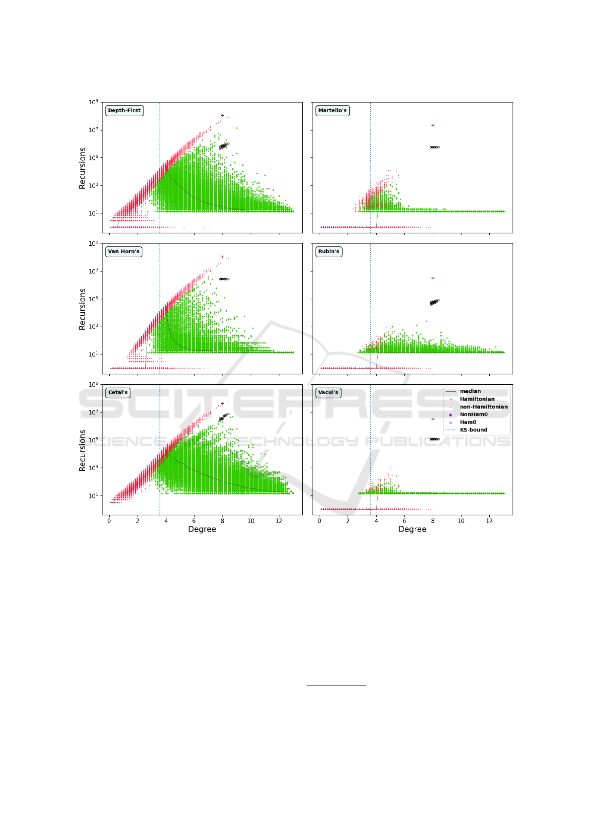
Figure 2: According to traditional views, the hardest Hamiltonian cycle problem instances lie close to its solvability phase

transition, the Koml

os-Szemer

edi-bound. Indeed this is true for large random ensembles, but a deliberate evolutionary search

for the hardest yes/no-instances found instances that are hard for all these algorithms, sometimes by several orders of magni-

tude than random ensembles (see markers for Ham

and NonHam

Karp, 1972) – the latter being Robert Tarjan, another

mastodont of computer science. His original publica-

tion seems hard to ﬁnd, but Garey and Johnson pro-

vide a proof of the Hamiltonian cycle problem’s NP-

completeness from the vertex cover problem. A di-

rect transformation to the satisﬁability problem (SAT)

is also possible, as shown for planar Hamiltonian cy-

cle problems in cubic graphs (which have maximum

vertex degree three)(Garey et al., 1976). Although

clever, the direct practicality could be compromised

by the large sizes of the Hamiltonian cycle problem

instances that can arise even from the transformation

of a single small SAT-instance. This principle, that in-

stance sizes need not hold under NP-complete trans-

formations is colloquially known as the ‘TommyGun

Theorem’.

Being NP-complete, the Hamiltonian Cycle prob-

lem has no known polynomial-time exact algorithm

An ‘exact algorithm’ for a decision problem such as

the Hamiltonian cycle problem, will always return a solu-

tion, given enough runtime.

Universally Hard Hamiltonian Cycle Problem Instances

107

In fact, the best upper bound was set by Richard Karp

himself, together with Michael Held, with a dynamic

programming algorithm that runs in O(n

) (Held

and Karp, 1962). Independently discovered and pub-

lished by Richard Bellman, it is still the fastest algo-

rithm for the worst-case instance, and hence has the

lowest known complexity – which is still exponential

(Bellman, 1962).

Although well-regarded, Held-Karp is by no

means the only exact algorithm for the Hamiltonian

cycle problem. In fact, a number of recursive back-

tracking algorithms have been devised through the

years. Plain depth-ﬁrst search was invented far be-

fore any modern day computer in 1882. As early as

1974, the far more sophisticated Rubin’s algorithm

already contained a surprising number of efﬁcient

subprocedures for non-Hamiltonicity checks (Rubin,

1974). Nine years later, an algorithm was proposed by

Sylvano Martello (Martello, 1983), who has a wide

track record with other NP-complete problems such

as (perfect) rectangle packing (Iori et al., 2021b; Iori

et al., 2021a; Iori et al., 2021c)(Braam and van den

Berg, 2022)(van den Berg et al., 2016). Martello’s

algorithm ’595’ is not particularly efﬁcient, but not

nearly as bad as Cetal’s algorithm, probably the most

inefﬁcient of them all (Cheeseman et al., 1991)(van

Horn et al., 2018).

Nevertheless, Cetal’s work had value: as an enor-

mous contribution to the awareness of hardness vari-

ation. An important note however, is that their ex-

periment on the traveling salesman problem instance

hardness was critically ﬂawed due to a roundoff er-

ror (Sleegers et al., 2020). Even so, Cetal’s assess-

ment on the other three NP-complete problems (in

particular the Hamiltonian cycle problem) that hard

instances reside close to the yes/no phase transition

still, holds up for large randomized sets. If only they

had used Frank Rubin’s algorithm from 20 years ear-

lier, or even just Van Horn’s from 2018 (which is just

a basic inversion of Cetal’s (van Horn et al., 2018)),

their results might have taken a much larger step for-

ward.

But the best performance award turned out to

be reserved for Basil Vandegriend & Joe Culberson

(abbreviated to “Vacul”), whose Vacul’s algorithm,

even better than Frank Rubin’s, was published in

1998, and corroborated that even for that algorithm,

the hardest problem instances were close to the phase

transition (Vandegriend and Culberson, 1998). Fi-

nally, a comprehensive comparative study by Joeri

Sleegers showed that all the algorithms are quite sim-

ilar: backtracking algorithms with degree priority,

pruning and check subroutines switched on or off.

Sleegers, aided by modern day computation power,

generated large ensembles of random graphs, which

he ran through all six backtracking algorithms

, tying

up earlier ﬁndings, showing that the hardest instances

for all these algorithms are close to the yes/no phase

transition (Sleegers and Van den Berg, 2021).

3 EVOLUTIONARY HARDNESS

So until 2020 the case for the Hamiltonian was crys-

tal clear: like all NP-complete problems, it has a

solvability phase transition, in this (rare) case exactly

characterized by the Koml

os-Szemer

edi bound (or

KS-bound), and the hardest instances, which are sig-

niﬁcantly harder than a given random instance, are lo-

cated very close to that bound for all major backtrack-

ing algorithms (Sleegers and Van den Berg, 2021).

But 21

century computing power was about to

throw a wrench in the machine, as Joeri Sleegers

was about to evolve Hamiltonian cycle problem in-

stances, making them as hard as possible using two

evolutionary algorithms. First, a fully stochastic

hillClimber was implemented; the algorithmic pro-

cess was as follows: a single mutation on the in-

cumbent hardest instance, which was retained if and

only if the mutant was harder or equally hard. Oth-

erwise, the mutation was reverted. Second, the

population-based plant propagation algorithm (PPA),

whose central idea is that ﬁtter individuals produce

many offspring with few mutations whereas unﬁtter

individuals produce fewer offspring with high muta-

bility, thus alledgedly “[balancing the forces of ex-

ploration and exploitation]” (Vrielink and van den

Berg, 2019). Since its introduction by Abdellah Salhi

and Eric Fraga (Salhi and Fraga, 2011), the paradigm

has seen a number of applications (Sulaiman et al.,

2018)(Sleegers and van den Berg, 2020a)(Sleegers

and van den Berg, 2020b)(Fraga, 2019)(Rodman

et al., 2018), as well as some spinoffs (Sulaiman

et al., 2016)(Paauw and van den Berg, 2019; Dijkzeul

et al., 2022)(Selamo

glu and Salhi, 2016)(Haddadi,

2020)(Geleijn et al., 2019). For the experiment, a

constant popSize = 10 was adopted, which produced

25 offspring every generation, which were distributed

and mutated as shown in table 1.

Table 1: The number and mutability of offspring produced

by PPA’s individuals are based on its ﬁtness rank (1 =

ﬁttest).

Rank 1 2 3 4 5 6 – 10

#offspring 6 5 4 3 2 1

#mutations 1 2 5 5 10 20

Source code is publicly available (Source, 2022).

ECTA 2022 - 14th International Conference on Evolutionary Computation Theory and Applications

108

Both evolutionary algorithms used three mutation

types with equal probability:

1. to insert an edge at a randomly chosen unoccu-

pied place in the graph,

2. to remove a randomly chosen existing edge from

the graph,

3. and to move an edge, which is effectively equal to

a remove mutation followed by an insert mutation

(on a different unoccupied place).

For the hillClimber runs, 20 randomly generated

graphs were evenly dispersed in terms of edge density,

ranging from 0 to

V ·(V −1) edges, corresponding to

edge densities ∈ {0%, 5%, 10%...95%}. For the PPA

runs, twenty initial populations with popSize = 10

were made along the same edge density intervals,

with all graphs in one population having the same

edge density. It should be noted that these densities

are ﬁxed only upon initialization, as the evolution-

ary algorithms are free to insert and remove edges

from graphs at every step of a run. The rationale be-

hind this choice of edge densities is that earlier results

could have been biased from the initialization on the

Koml

os-Szemer

edi bound. This spread out approach

would cover a much wide area of the state space – at

least in terms of initial conditions. For the end results

however, it did not make much of a difference.

From these evenly distributed initial positions,

both algorithms ran 3000 function evaluations, corre-

sponding to 3000 generations for the stochastic hill-

Climber, but 120 generations of PPA. For the hardest

instance, both algorithms converged on the same in-

stance, a highly regular wall-and-clique-graph (Fig-

ure 1), not having a Hamiltonian cycle. For yes-

instances however (graphs which do have a Hamil-

tonian cycle) the hardest was in fact not a solitary

graph, but rather a constellation of 27 equihard non-

isomorphic graphs which were connected by one-

bit mutations: the Hamiltonian plateau (Figure 1)

(Sleegers and van den Berg, 2022). In this paper,

we will show that these evolutionarily found instances

are not only hard for Vacul’s algorithm, but possess a

more universal hardness.

4 EXPERIMENT & RESULTS

The hardest evolutionarily found instances (as seen

in Figure 1) are all 14-vertex graphs. The reason

that Sleegers & Van den Berg originially used such

instances, is that because the evolutionary algorithm

constantly pushes for hardness, measured through the

number of recursions for the most efﬁcient known

backtracking algorithm, even a single function eval-

uation of the evolutionary algorithm can require

millions of recursions, which consumes incredible

amounts of computational power over the evolution-

ary trajectory, especially for population-based algo-

rithms.

For a fair comparison, we generated an ensemble

of random graph which also have V = 14 vertices.

The maximum number of edges that a V = 14 graph

instance can hold is

· 14 · 13 = 91, so for the ran-

dom ensemble, we generated 1000 graphs for each

E ∈ [1, 91], meaning we covered the entire edge den-

sity range with a set of 91,000 graphs. We will call

this ensemble Rand91K, and all graphs are publicly

available (Source, 2022). Then, we added the single

nonHam

graph and the 27 Ham

graphs, the hardest

no- and yes-instances as found by our evolutionary al-

gorithms. After that, each of these 91028 problem in-

stances was decided in six experiments, one for each

recursive algorithm, and the results can be found in

Figure 2.

Of the 91,000 instances in Rand91K, 61720 were

Hamiltonian, whereas 29280 were not. These num-

bers might seem counterintuitive, but one should re-

alize that the KS-bound for Hamiltonicity in a graph

of V vertices scales as

V ln(V ) +

V ln(ln(V )),

whereas possible number of edges scales as

V (V −

1). The combinatorial peak lies somewhat lower at

V (V − 1), but even for very modest numbers of

V , there are far more T RUE-instances than FALSE-

instances for the Hamiltonian cycle problem. For

V = 10, approximately 73% of all existible instances

are Hamiltonian; for V = 14, the percentage is al-

ready 93%

. It is paradoxical but true that for this NP-

complete decision problem, nearly every existable in-

stance is a yes-instance.

Nonetheless, NP-complete classiﬁcation relies on

the guarantee of exactness; it follows that all 91,000

instances were decided upon by all six algorithms, the

results of which can be found in Table 2 in columns

2-5. Results for the evolutionarily found hard in-

stances are in the ﬁnal two columns. In line with pre-

vious results, the three algorithms with pruning and

check routines (bottom three rows) outperform the

more basic algorithms. In addition, the evolutionar-

ily found Ham

and NonHam

are very hard for all

backtracking algorithms, even though the difference

is less acute for the basic algorithms, which are in-

efﬁcient on a large part of the Rand91K set to begin

with.

For almost all algorithms, the nonHam

was

harder then every instance in the 91,000 random graph

Numbers in this study differ a bit because we forced

1,000 graphs for every possible edge degree.

Universally Hard Hamiltonian Cycle Problem Instances

109

Table 2: The hardest evolutionarily generated yes- and no-instances (Ham

and NonHam

) for Vacul’s algorithm are among

the hardest instances for all backtracking algorithms used in this study, even though the discrepancies are much more acute

for the three more advanced algorithms (values of µ and σ are rounded). Are Ham

and NonHam

universally hard instances

for the problem?

Algorithm median rec. µ recursions σ recursions max. recursions max. rec. Ham

rec. NonHam

Depth-ﬁrst 25 13,841 392,694 78,238,081 994,086 104,845,861

Van Horn’s 14 11,755 375,779 78,378,266 2,594,148 104,845,861

Cetal’s 71 11,047 307,582 64,760,949 7,321,408 41,803,191

Martellos 14 13 86 11,483 554,760 21,978,181

Rubin’s 14 11 14 2,528 75,894 3,091,141

Vacul’s 14 10 8 967 109,632 3,091,141

ensemble. For Vacul’s, Martello’s and Rubin’s, it was

3197 times, 1914 times and 1223 times harder than

the hardest graph in the ensemble, which was non-

Hamiltonian in Vacul’s and Martello’s, but Hamilto-

nian in Rubin’s case, surprisingly enough. A quick-

and-dirty explanation might be that nonHam

nar-

rowly ‘dodges’ the pruning and test procedures that

these algorithms have, leaving it up to a high number

of recursions.

For the non-pruning non-check algorithms, results

were a lot less conclusive: in both plain depth-ﬁrst

and Van Horn’s, nonHam

was ‘only’ 1.34 times

harder than the hardest (non-Hamiltonian) instance in

the ensemble. For Cetal’s, it wasn’t even the hard-

est, but 0.65 times the hardness of the hardest (non-

Hamiltonian) instance in the ensemble, and 1.43 times

harder than the second hardest (non-Hamiltonian) in-

stance in the ensemble. This appears largely a testa-

ment of the efﬁciency of the algorithms with checks

and pruning, or, as Steven Skiena once said: “Clever

pruning can make short work of surprisingly hard

problems” (Skiena, 1998).

For the 27 graphs of Ham

set, the results were

far less resounding, but still a clear distinction could

again be noticed for the three algorithms with checks

and pruning. For the highly efﬁcient algorithm by

Vacul, the entire Ham

set was 113 times harder

than the hardest instance from the Rand91K-set. For

Rubin’s algorithm, the 27 instances of Ham

set

no longer form a plateau. They are nonetheless a

hard set, requiring between 75,894 and 37,824 recur-

sions, still 15 times more than the hardest Rand91K-

instance at 2528 recursions. For Martello’s, the 27

graphs of Ham

do constitute a plateau, whose in-

stances are 48 times harder than the hardest graph

from Rand91K.

For the non-pruning non-check algorithms, the

Ham

was still a hard set of instances, but results

were a lot messier. In Van Horn’s, no less than 60

instances (58 non-Hamiltonian and 2 Hamiltonian)

from the Rand91K-set were harder than Ham

. For

Cetal’s algorithm, the 81 hardest instances contained

the entire Ham

-set, the nonHam

and another 53

Rand91K-instances. For depth-ﬁrst, the Ham

-set,

the nonHam

-instance and 421 Rand91K-instances

made up the 449 hardest instances. The quick and

dirty explanation is that this algorithm underperforms

on the Ham

-set, but underperforms even worse on

some of the Rand91K-instances. Nonetheless the dif-

ference with the nonHam

, which is the almost ex-

clusively hardest instance for all studied algorithms,

is stark.

5 CONCLUSIONS

The current results present some evidence that the

hardest Hamiltonian cycle instances for one exact

backtracking algorithm, are hard(est) for other exact

backtracking algorithms too. The contrast is greatest

in the most efﬁcient algorithms, but that has more to

do with the inefﬁciency of the other backtracking al-

gorithms. Still, we must not close our eyes to thenu-

ances in the narrative: for some inefﬁcient algorithms,

still harder instances exist, be it very few. Nonethe-

less, nonHam

and the Ham

-set can be considered

almost universally hard for backtracking algorithms.

The fact that these hardest instances do not appear

in large random ensembles such as the Rand91K-set

also begs the question what makes the Hamiltonian

cycle problem NP-complete. Is it possible that efﬁ-

cient backtrackers solve all but a very small number

of instances, which can be listed in a table? And if so,

how does the table scale under increasing V ? Con-

sidering their structural regularity, they might even

have a short algorithmical description. We should fur-

ther reﬁne these instances. Although somewhat out

of fashion, it is clear that the class of recursive back-

tracking algorithms has not yet revealed all of its se-

crets.

REFERENCES

Bellman, R. (1962). Dynamic programming treatment of

the travelling salesman problem. Journal of the ACM

(JACM), 9(1):61–63.

ECTA 2022 - 14th International Conference on Evolutionary Computation Theory and Applications

110

Braam, F. and van den Berg, D. (2022). Which rectangle

sets have perfect packings? Operations Research Per-

spectives, page 100211.

Cheeseman, P. C., Kanefsky, B., and Taylor, W. M. (1991).

Where the really hard problems are. In IJCAI, vol-

ume 91, pages 331–340.

Dijkzeul, D., Brouwer, N., Pijning, I., Koppenhol, L., and

Van den Berg, D. (2022). Painting with evolutionary

algorithms. In International Conference on Compu-

tational Intelligence in Music, Sound, Art and Design

(Part of EvoStar), pages 52–67. Springer.

Fraga, E. S. (2019). An example of multi-objective opti-

mization for dynamic processes. Chemical Engineer-

ing Transactions, 74:601–606.

Garey, M. R. and Johnson, D. S. (2002). Computers and

intractability, volume 29. wh freeman New York.

Garey, M. R., Johnson, D. S., and Tarjan, R. E. (1976). The

planar hamiltonian circuit problem is np-complete.

SIAM Journal on Computing, 5(4):704–714.

Geleijn, R., van der Meer, M., van der Post, Q., and van den

Berg, D. (2019). The plant propagation algorithm on

timetables: First results. EVO* 2019, page 2.

Gent, I. P. and Walsh, T. (1996). The tsp phase transition.

Artiﬁcial Intelligence, 88(1-2):349–358.

Haddadi, S. (2020). Plant propagation algorithm for nurse

rostering. International Journal of Innovative Com-

puting and Applications, 11(4):204–215.

Hayes, B. (1997). Computing science: Can’t get no satis-

faction. American scientist, 85(2):108–112.

Held, M. and Karp, R. M. (1962). A dynamic program-

ming approach to sequencing problems. Journal of

the Society for Industrial and Applied Mathematics,

10(1):196–210.

Iori, M., De Lima, V., Martello, S., and M., M. (2021a).

2dpacklib: a two-dimensional cutting and packing li-

brary (in press). Optimization Letters.

Iori, M., de Lima, V. L., Martello, S., Miyazawa, F. K., and

Monaci, M. (2021b). Exact solution techniques for

two-dimensional cutting and packing. European Jour-

nal of Operational Research, 289(2):399–415.

Iori, M., de Lima, V. L., Martello, S., and Monaci, M.

(2021c). 2dpacklib.

Karp, R. M. (1972). Reducibility among combinatorial

problems. In Complexity of computer computations,

pages 85–103. Springer.

Karp, R. M. (2008). Reducibility among combinatorial

problems. 50 Years of Integer Programming 1958–

2008, page 219.

Koml

os, J. and Szemer

edi, E. (1983). Limit distribution for

the existence of hamiltonian cycles in a random graph.

Discrete Mathematics, 43(1):55–63.

Larrabee, T. and Tsuji, Y. (1992). Evidence for a satisﬁa-

bility threshold for random 3CNF formulas. Citeseer.

Martello, S. (1983). Algorithm 595: An enumerative al-

gorithm for ﬁnding Hamiltonian circuits in a directed

graph. ACM Transactions on Mathematical Software

(TOMS), 9(1):131–138.

Paauw, M. and van den Berg, D. (2019). Paintings,

polygons and plant propagation. In International

Conference on Computational Intelligence in Music,

Sound, Art and Design (Part of EvoStar), pages 84–

97. Springer.

Rodman, A. D., Fraga, E. S., and Gerogiorgis, D. (2018).

On the application of a nature-inspired stochastic

evolutionary algorithm to constrained multi-objective

beer fermentation optimisation. Computers & Chemi-

cal Engineering, 108:448–459.

Rubin, F. (1974). A search procedure for hamilton paths and

circuits. Journal of the ACM (JACM), 21(4):576–580.

Salhi, A. and Fraga, E. S. (2011). Nature-inspired optimi-

sation approaches and the new plant propagation algo-

rithm.

Selamo

glu, B.

I. and Salhi, A. (2016). The plant propaga-

tion algorithm for discrete optimisation: The case of

the travelling salesman problem. In Nature-inspired

computation in engineering, pages 43–61. Springer.

Skiena, S. S. (1998). The algorithm design manual. page

247.

Sleegers, J., Olij, R., van Horn, G., and van den Berg, D.

(2020). Where the really hard problems aren’t. Oper-

ations Research Perspectives, 7:100160.

Sleegers, J. and van den Berg, D. (2020a). Looking for

the hardest hamiltonian cycle problem instances. In

IJCCI, pages 40–48.

Sleegers, J. and van den Berg, D. (2020b). Plant propaga-

tion & hard hamiltonian graphs. Evo* 2020, page 10.

Sleegers, J. and Van den Berg, D. (2021). Backtracking

(the) algorithms on the hamiltonian cycle problem. In-

ternational Journal On Advances in Intelligent Sys-

tems, 14:1–13.

Sleegers, J. and van den Berg, D. (2022). The hardest hamil-

tonian cycle problem instances: the plateau of yes and

the cliff of no. SCSC. (In press.).

Source (2022). Publicly accessible source code, in-

stances & results. https://github.com/Joeri1324/

Universally-Hard-Hamiltonian-Cycle-Problem-Instances.

Last accessed june 18

, 2022.

Sulaiman, M., Salhi, A., Fraga, E. S., Mashwani, W. K., and

Rashidi, M. M. (2016). A novel plant propagation al-

gorithm: modiﬁcations and implementation. Science

International, 28(1):201–209.

Sulaiman, M., Salhi, A., Khan, A., Muhammad, S., and

Khan, W. (2018). On the theoretical analysis of the

plant propagation algorithms. Mathematical Problems

in Engineering, 2018.

Van Den Berg, D. and Adriaans, P. (2021). Subset sum

and the distribution of information. In Proceedings of

the 13th International Joint Conference on Computa-

tional Intelligence, pages 135–141.

van den Berg, D., Braam, F., Moes, M., Suilen, E., Bhulai,

S., et al. (2016). Almost squares in almost squares:

solving the ﬁnal instance.

van Horn, G., Olij, R., Sleegers, J., and van den Berg, D.

(2018). A predictive data analytic for the hardness of

hamiltonian cycle problem instances. DATA ANALYT-

ICS 2018, page 101.

Vandegriend, B. and Culberson, J. (1998). The gn, m

phase transition is not hard for the Hamiltonian cycle

problem. Journal of Artiﬁcial Intelligence Research,

9:219–245.

Vrielink, W. and van den Berg, D. (2019). Fireworks algo-

rithm versus plant propagation algorithm.

Universally Hard Hamiltonian Cycle Problem Instances

111