Investigating Prediction Models for Vehicle Demand in a Service Industry

Ahmed Alzaidi, Siddhartha Shakya and Himadri Khargharia

EBTIC, Khalifa University, Abu Dhabi, U.A.E.

Keywords:

Machine Learning, Demand Forecasting, Resource Management.

Abstract:

Demand prediction is an important part of resource management. Higher forecasting accuracy leads to bet-

ter decision taking capabilities, especially in a competitive service-based business such as telecommunication

services. In this paper, a telecommunication service provider’s data on the use of vehicles by their employees

is analyzed and used to forecast the vehicle booking demand for the future at different geographical locations.

We implement multiple forecasting models and investigate the effect on forecasting accuracy of two predic-

tion strategies, namely the Direct multi-step forecasting strategy (DMS) and the Rolling mechanism strategy

(RMS). Moreover, the effect of different external inputs such as temperatures and holidays were tested. The

results show that both DMS and RMS can be used to forecast vehicle demand, with the highest improvement

in forecasting achieved through the addition of the holiday input, particularly by using the RMS strategy in

the majority of the cases.

1 INTRODUCTION

Flawless operation with constrained supply requires

an effective resource management strategy. The con-

tinuum in the supply can be ensured through the ac-

curate prediction of the demand with the exploita-

tion of historical data. Businesses such as telecom-

munication, utilities, retail, hotels, etc, recognize the

importance of accurate forecasting for demand espe-

cially when the supply is constrained. Indeed, oper-

ational efﬁciency and sustainable revenue growth in

businesses, with limited supply, are sensitive to poor

demand predictions (Azadeh et al., 2015). Hence,

corporations are keen to exploit machine learning and

other artiﬁcial intelligence methods for producing a

more accurate forecast. Higher operational efﬁciency

improves the quality of service leading to higher lev-

els of customer satisfaction.

However, in the service industry, maintaining ser-

vice standards is coupled with the availability of re-

strained resources to meet the demand. Based on the

types of industries, there could be many different re-

sources involved in providing services, such as vehi-

cles, specialized technical equipment, hardware loads

for when the device can sustain a certain limit of loads

(Herrer

ıa-Alonso et al., 2021), rooms or beds for in-

dividuals in hotels (Lee, 2018) or hospitals (Deschep-

per et al., 2021; Goic et al., 2021), etc. Generally,

the demand is predicted after analysis of the histori-

cal demand data besides other correlated data such as

weather, seasonality, geography, etc, to enhance the

forecasting accuracy and thus better manage the avail-

able resources. Different strategies such as Rolling

mechanism forecasting strategy (RMS) (Mu et al.,

2019), Direct multi-step forecasting strategy (DMS)

(Shi and Yeung, 2018) can be adopted by different

forecasting techniques for improving the accuracy.

Businesses such as utility companies, telecommu-

nication service providers, and car sharing companies

use vehicles to provide services to their consumers.

They normally own a ﬂeet of vehicles. An employee

can request a vehicle for a certain hour or day and se-

lect a pick up location from the available locations.

This creates a record of the historical usage data in

different parking hubs and keeps track of the vehicles.

This historical usage data allows visualization of the

demand at respective parking hubs and can also be ex-

ploited to forecast the future demand for the vehicles

(Liu et al., 2021a; M

uller and Bogenberger, 2015; Yu

et al., 2020), thus ensuring their availability upon the

requested booking date and enhancing operational ef-

ﬁciency.

In this work, we focus on the data provided by

our partner telecommunication service provider that

keeps a ﬂeet of vehicles at different parking hubs. The

engineers can book the vehicles on a daily basis to

perform the tasks allocated to them. The choice of

parking hub for booking may depend on the starting

Alzaidi, A., Shakya, S. and Khargharia, H.

Investigating Prediction Models for Vehicle Demand in a Service Industry.

DOI: 10.5220/0011527400003332

In Proceedings of the 14th International Joint Conference on Computational Intelligence (IJCCI 2022), pages 359-366

ISBN: 978-989-758-611-8; ISSN: 2184-3236

359

location of the engineer as well as the locations of the

tasks that they are performing. Hence, the demand for

vehicles can be different for different dates even for

the same parking hub. We investigate and evaluate

different forecasting strategies and forecasting mod-

els with the aim of accurately predicting the vehicle

booking demand for each parking hub. The ultimate

goal is to build a tool that can be used to manage re-

sources on a daily basis. We perform experiment with

the historical data provided by our partner telecom

and analyze the results to identify the best performing

method. Real-world data on the historical bookings

were combined with additional data involving ofﬁcial

holiday and temperature data to improve the accuracy.

We show the effectiveness of the tested methods and

provide a detail analysis of the results.

The rest of the paper is organized as follows. Sec-

tion 2 reviews related works, particularly focusing on

works, where the RMS and DMS were used and how

other factors were incorporated into the forecast. Sec-

tion 3 explains the data and the methods used. Section

4, presents the experiments and interprets the results,

and ﬁnally, section 5 provides a conclusion to the ﬁnd-

ings.

2 BACKGROUND

There are many use cases where DMS and RMS were

used for forecasting. For example, DMS was ex-

ploited to predict energy prices and wind power with a

radial-basis functional network (Khalid, 2019). It was

found to outperform the recursive forecasting strat-

egy when used with a random forest algorithm for

wind speed prediction (Vassallo et al., 2020). An-

other study implemented the DMS with XGBoost al-

gorithm to predict the state of charge and terminal

voltage in lithium-ion batteries that are exposed to dif-

ferent loads (Dineva et al., 2021). The trafﬁc speed

was predicted using DMS with an ensemble model

(Feng et al., 2021).

Many forecasting scenarios depend on the short

window from the recent past. Short-term predictions

of water levels in different water channels in a river

located in China were tested via the implementation

of an RMS with Long short-term memory (LSTM)

algorithm (Liu et al., 2021b). In (Yuan et al., 2021),

authors created an ensemble model composed of dif-

ferent models that used LSTM with RMS to forecast

the intensity of typhoons. A comparative study is

done in (Yuan et al., 2019) that found Convolutional

Long Short-Term Memory with Ensemble Empiri-

cal Mode Decomposition (EEMD-ConvLSTM) with

RMS to be more robust than the one-step forecasting

models exploiting Global Forecast System, Medium

Range Forecast (MRF), Model Ensemble Members

(ENSM) in forecasting North Atlantic Oscillation in-

dex. While (Du et al., 2016) uses RMS forecasting

with different algorithms to predict wind speed. The

demand was predicted with LSTM through the RMS

forecasting approach (Wang et al., 2021a).

In (Surakhi et al., 2021) the time lag inﬂuence on

the accuracy of the predictions is investigated and it is

found that the selection of time lags affect the accu-

racy signiﬁcantly due to correlation strength between

the selected time lag values. The historical values

(time lags values) of electricity consumption alone

were found to be able to eliminate the need for ad-

ditional inputs such as weather data as they already

captured the effect of weather data, and emphasized

the need to select the optimal number of lagged val-

ues via genetic algorithms(Bouktif et al., 2018). Both

(Bakker et al., 2014; Wang et al., 2021b) found that

using weather input improved the forecasting accu-

racy. The weather, holiday, and accident were used in

the form of one-hot encoding as additional input to the

trafﬁc forecasting models and were found to enhance

the predictions (Sun et al., 2020).

3 METHODOLOGY

Historical vehicle booking records of 91 days for 10

parking locations (hereafter referred to as parking 1,

parking 2, etc) were acquired. The data represent the

number of vehicles booked for the selected date at

each station. It is a continuous univariate time se-

ries data for the vehicle booking at different parking

hubs. As an example, bookings for parking hubs 3,

5, and 9 are shown in Figure. 1, which shows that

there is a shared pattern in booking demand except

for the period between the 16

of July and the 30

July where the booking requests dropped abnormally

and then raised sharply afterward. This pattern is ob-

served in most of the parking hubs data with the dif-

ference being the total booking request. Comparing

the different parking hubs, we found that the booking

request is lowest in parking hub 5 during all the peri-

ods. On the other hand, we found that parking hubs 8

and 9 are alternate as the most booked parking hub.

The weather plays an important role in everyday

transportation decisions and might affect the book-

ing of vehicles at different parking hubs. The fore-

casted temperature for the period between 15

May

and 17

August 2021 was collected (Figure. 2). It can

be observed that the temperature gradually increased

throughout the data.

The publicly announced holidays are shown in ta-

NCTA 2022 - 14th International Conference on Neural Computation Theory and Applications

360

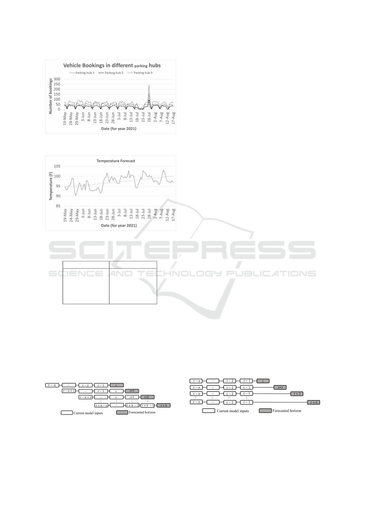
Figure 1: Vehicle bookings by date for parking hubs 3, 5

and 9.

Figure 2: Temperature forecast data in Fahrenheit.

Table 1: Public holiday dates and the corresponding day of

the week.

Date Day of the week

19 July 2021 Monday

20 July 2021 Tuesday

21 July 2021 Wednesday

22 July 2021 Thursday

12 August 2021 Thursday

ble 1. The public holidays apply to all the sectors,

thus inﬂuencing the booking levels. The holiday dates

in the tables match the sudden changes in the trends

within the booking shown in Figure. 1 which indicate

a correlation between the holiday and vehicle book-

ings.

3.1 Rolling Mechanism Forecasting

(RMS)

Figure 3: The working concept of RMS.

RMS is a forecasting strategy that utilizes the recent

trends in data to forecast future values which are re-

ferred to as forecasting horizons (Mu et al., 2019). All

the values in the forecasting horizons are predicted us-

ing the same model that is ﬁtted to take a ﬁxed rolling

window of inputs when no external factors are consid-

ered. Figure 3 demonstrates the concept of the rolling

mechanism. When the ﬁrst period in the horizon is

predicted, the ﬁxed window of input is coming from

real data, yet when the second period is predicted the

ﬁrst-period prediction is added as the most recent in-

put to the rolling window, and the input furthest from

the value to be predicted is removed. This new input

window is used to predict the second period. When

the third period is predicted the second-period predic-

tion is used as the most recent input and the value

furthest from the third period is removed. To explain

the concept mathematically, let B be the set of all the

vehicle bookings in a parking hub. Then we assume

rms

⊂ B to represent a subset of bookings considered

for RMS, such that

rms

= {b

t+h−i

|1 ≤ i ≤ n, ∀b

t+h−i

∈ B} (1)

where b

t+h−i

represents the booking entry from

set B, n represents the size of the rolling window, h

represents the forecasting time step, t represents the

time step for the ﬁrst forecasted period, then

t+h

= F (B

rms

) (2)

where, b

t+h

is the foretasted booking for the time

step h and F is the forecasting model. This forecast-

ing strategy has the advantage of adapting to changes

in data and the training phase of the model assigns

importance to the input values based on their proxim-

ity from the predicted horizon, thus adapting to data

trends. Additionally, the method is computationally

less expensive as one model is needed for predicting

all values in the horizon H. However, because the pre-

vious prediction is used in the forecast of other hori-

zons, the error is accumulated as the prediction steps

increase.

3.2 Direct Multi Step Forecasting

Strategy (DMS)

Figure 4: The working concept of DMS.

In DMS, each step ahead is predicted independently

via a different model. Each period is predicted via

Investigating Prediction Models for Vehicle Demand in a Service Industry

361

a separate model which is trained and validated us-

ing a modiﬁed data set speciﬁc to that perdition pe-

riod, yet all the models use the exact same input to

predict their corresponding periods (Shi and Yeung,

2018). The concept of DMS forecasting is illustrated

in Figure 4. To explain the DMS mathematically, lets

assume B

dms

⊂ B to represent a subset of bookings

considered for DMS, such that

dms

= {b

t−i

|1 ≤ i ≤ n, ∀b

t−i

∈ B} (3)

where b

t−i

represent the booking entry from set B

and n represent the size of the input window, t repre-

sents the time step of the ﬁrst forecasted period, then

t+h

= θ

dms

) (4)

where,b

t+h

is the foretasted booking for the time

step h and θ

is the model speciﬁc for predicting the

booking b

t+h

at the forecasted time step h. The DMS

does not cause error accumulation as predicted hori-

zons are not used as input to predict further horizons

(Dossani, 2022). This advantage in DMS forecasting

made it interesting to test for booking demand fore-

casting. However, as all the models use the same in-

puts, the DMS does not capture the relationship be-

tween the different time steps of the modeled case

(Taieb et al., 2012). Furthermore, creating an indi-

vidual model for each horizon is a computationally

expensive process that becomes a liability when the

number of the forecasted horizon is large.

3.3 Machine Learning Algorithms

In this paper, we implement different machine

learning algorithms with multiple parameter set-

tings to forecast the booking demand. They in-

cludes K-nearest neighbour regressor (KNN), deci-

sion tree (DT), ridge regression (RR), Lasso Re-

gression (Lasso), liner regression (LR), random for-

est (RF), neural network (NN), stochastic gradi-

ent descent (SGD), support vector regressor (SVR)

(James et al., 2021), Gradient Boosting (Friedman,

2001) (GBoost), extrem gradiant boosing (Chen and

Guestrin, 2016) (XGBoost), light gradient boosting

machine (LGBM) (Ke et al., 2017), ExtraTreesRe-

gressor (Geurts et al., 2006), MLPRegressor (Hornik

et al., 1989) and ElasticNet (Zou and Hastie, 2003).

Due to limited space, we do not go into details of

these algorithms. Interested readers are reffered to

(James et al., 2021).

3.4 Model Formulation

It can be observed in Figure 1 that each parking hub

experience different booking level. Hence, we model

Table 2: Input Forms.

SL No Input Form Name D W T H

1 D7W0 7 0 - -

2 D14W0 14 0 - -

3 D6W3 6 3 - -

4 D7W0T 7 0 * -

5 D14W0T 14 0 * -

6 D6W3T 6 3 * -

7 D7W0T1 7 0 1 -

8 D14W0T1 14 0 1 -

9 D6W3T1 6 3 1 -

10 D7W0T3 7 0 3 -

11 D14W0T3 14 0 3 -

12 D6W3T3 6 3 3 -

13 D7W0H 7 0 - *

14 D14W0H 14 0 - *

15 D6W3H 6 3 - *

16 D7W0TH 7 0 * *

17 D14W0TH 14 0 * *

18 D6W3TH 6 3 1 *

19 D7W0T1H 7 0 1 *

20 D14W0T1H 14 0 1 *

21 D6W3T1H 6 3 1 *

22 D7W0T3H 7 0 3 *

23 D14W0T3H 14 0 3 *

24 D6W3T3H 6 3 3 *

each parking hub separately, i.e, for each parking hub,

we built 2 models (RMS and DMS), for each conﬁgu-

ration of input features, to test the effect of the differ-

ent model conﬁgurations on the forecasting accuracy.

In total, 24 feature conﬁgurations including different

external features and with different lag setups were

tested for each of the two models. Data for each of

these conﬁgurations were ﬁtted on multiple machine

learning algorithms as listed in the previous section,

and for multiple different parameter settings of these

algorithms. The result for the model with the best

accuracy was taken as the result for that input conﬁg-

uration.

3.5 Data Preparation

In RMS, the target needs to be the booking period

directly after the last booking period input. On the

other hand, the DMS requires a speciﬁc data set for

each predicted period, such that each period model

is trained to predict multiple periods ahead with the

same input used in the other models. Fortunately,

the RMS input data can be modiﬁed to ﬁt the DMS

requirement via shifting the target, thus training the

models to predict different steps ahead using the same

input.

NCTA 2022 - 14th International Conference on Neural Computation Theory and Applications

362

As shown in Table 2, 24 data inputs were gen-

erated for each of the parking hubs, termed input

forms, that represent different combinations of day

lags, week lags, temperature lags, and holidays. The

number after the D indicates the day lag, W indicates

the week lag, T indicates temperature input lag and H

indicates holiday inputs. If there was no number after

the T, this means that the temperature for the target

day was added to the inputs. Also ’-’ in the column

T and H represent the corresponding parameter was

not used, and ’*’ represent only the value for the tar-

get day was used in the input. Additionally, the day

of the week of the target date was used as an extra in-

put feature, encoded with one-hot encoding, creating

7 more binary inputs.

4 EXPERIMENTS AND RESULTS

In this section, the accuracy of RMS is compared to

DMS with different input forms and external input

combinations as shown in Table 2. Weighted abso-

lute percentage error (WAPE) was used as a measure

of accuracy. The data for the last 7 days were used

as a test set to calculate the accuracy. The model that

achieved the best WAPE accuracy was selected and

reported back with the results.

The KN, XGBoost , LGBM and RF all used

the default hyper parameters.The RF was tested

further through 13 different combination of max-

imum tree depth and number of estimator of

[(5,10),(5,15),(5,50),(7,80),(7,100),(7,120),(9,10),

(9,150), (11,10),(11,15),(11,100),(11,500),(13,700)]

respectively. DT algorithms was tested using 6

different maximum tree depths of 5, 7, 10, 15

and 20. The gradient boosting was tested with 11

different combination of hyper parameters, out of

which 7 combination only used number of estimators

and maximum depth with the respective values of

[(500,11),(500,3),(500,5),(100,11),(100,12),(100,13),

(100,14)]. The other combinations added the sub

sample parameter. The hyper parameter com-

bination in the respective order of number of

estimator , maximum depth and sub sample was

[(25,5,1),(30,5,1),(40,5,1,),(100,11,1)].

To make the results more comparable and readable

we present the model’s result in the form of accuracy

% as 1 − WAPE, for all the different cases tested in

both the RMS and DMS. The result of demand pre-

diction across the 10 parking hubs for the lagged input

forms D7W0, D14W0, and D6W3 with and without

the cases of the temperature input that is added as the

temperature of the target day (T), lagged temperature

of 1 day with the target day (T1) and lagged temper-

ature of 3 days with the target day (T3) are presented

on tables 3, 4, 5 and 6. The tables report the perfor-

mance results of the models in both the RMS and the

DMS for all the forms. The models in tables 3 and

4 did not use a holiday input and the variation in ac-

curacy is presented in a boxplot (Figure 5) comparing

the RMS versus the DMS approach in all the data in-

puts forms. Similarly, tables 5 and 6 present the per-

formance results for the models that used the Holiday

input while Figure 6 present a comparative visualiza-

tion of the model’s performance in both the RMS and

DMS cases for the different combinations of inputs.

4.1 Models Performance

Table 3: 1-WAPE results for the different parking hub mod-

els using DMS and RMS without a holiday input and using

the basic forms and the basic forms with temperature inputs.

RMS DMS

Form D7W0 D14W0 D6W3 D7W0 D14W0 D6W3

Parking hub1 86.95 88.35 86.9 92.09 90.47 89.46

Parking hub2 85.58 84.6 90.43 84.06 91.82 91.92

Parking hub3 88.12 88.38 85.87 89.65 88 72.19

Parking hub4 75.94 83.53 73.33 76.11 80.65 81.73

Parking hub5 77.15 76.3 80.91 77.04 86.29 69.95

Parking hub6 83.72 83.68 84.04 83.84 77.53 75.53

Parking hub7 90.77 93 92.29 92.52 83.17 86.96

Parking hub8 89.44 87.94 89.57 87.67 85.1 84.95

Parking hub9 84.48 86.88 86.95 85.84 88.78 85.72

Parking hub10 82 84.66 83.7 80.44 88.96 83.44

Average 84.41 85.73 85.4 84.93 86.08 82.18

Stdev 4.67 4.16 5.15 5.49 4.28 6.97

Form D7W0T D14W0T D6W3T D7W0T D14W0T D6W3T

Parking hub1 85.84 88.22 86.35 94.46 87.45 85.38

Parking hub2 86.36 83.89 87.57 83.11 87.29 93.36

Parking hub3 86.17 87.94 85.87 85.98 85.18 79.25

Parking hub4 78.95 80.72 75.34 72.73 76.2 84.7

Parking hub5 81.71 77.18 82.11 75.7 85.77 77.82

Parking hub6 82.32 81.47 83.54 77.01 75.89 74.22

Parking hub7 89.62 91.56 91.72 86.31 82.63 88.66

Parking hub8 89.17 89.01 90.18 88.34 88.21 83.76

Parking hub9 85.16 86.3 86.66 87.86 83.42 84.87

Parking hub10 82.27 84.31 84.39 80.37 91.74 78.98

Average 84.76 85.06 85.37 83.19 84.38 83.1

Stdev 3.23 4.16 4.32 6.36 4.82 5.35

We can notice that, RMS results are more consistent

in comparison to the DMS forecasting when the holi-

day parameter was not used (Table 3 and 4). The dif-

ferent data input forms did not affect the RSM perfor-

mance as much as the DMS and the temperature input

did not signiﬁcantly contribute to the improvement of

results. For the RMS, the D7W0 input accuracy im-

proved slightly when the temperature input of the tar-

get day or the temperature input of 1-day lag is added

to the RMS models while the opposite is observed for

input forms D14W0 and D6W3 for the prior condi-

tions. When a temperature lag of 3 was used, the

performance recorded was the lowest for all the input

forms. In the DMS case, the input forms D7W0 and

D14W0 experienced lower accuracy as more temper-

ature inputs were added. The only exception was for

Investigating Prediction Models for Vehicle Demand in a Service Industry

363

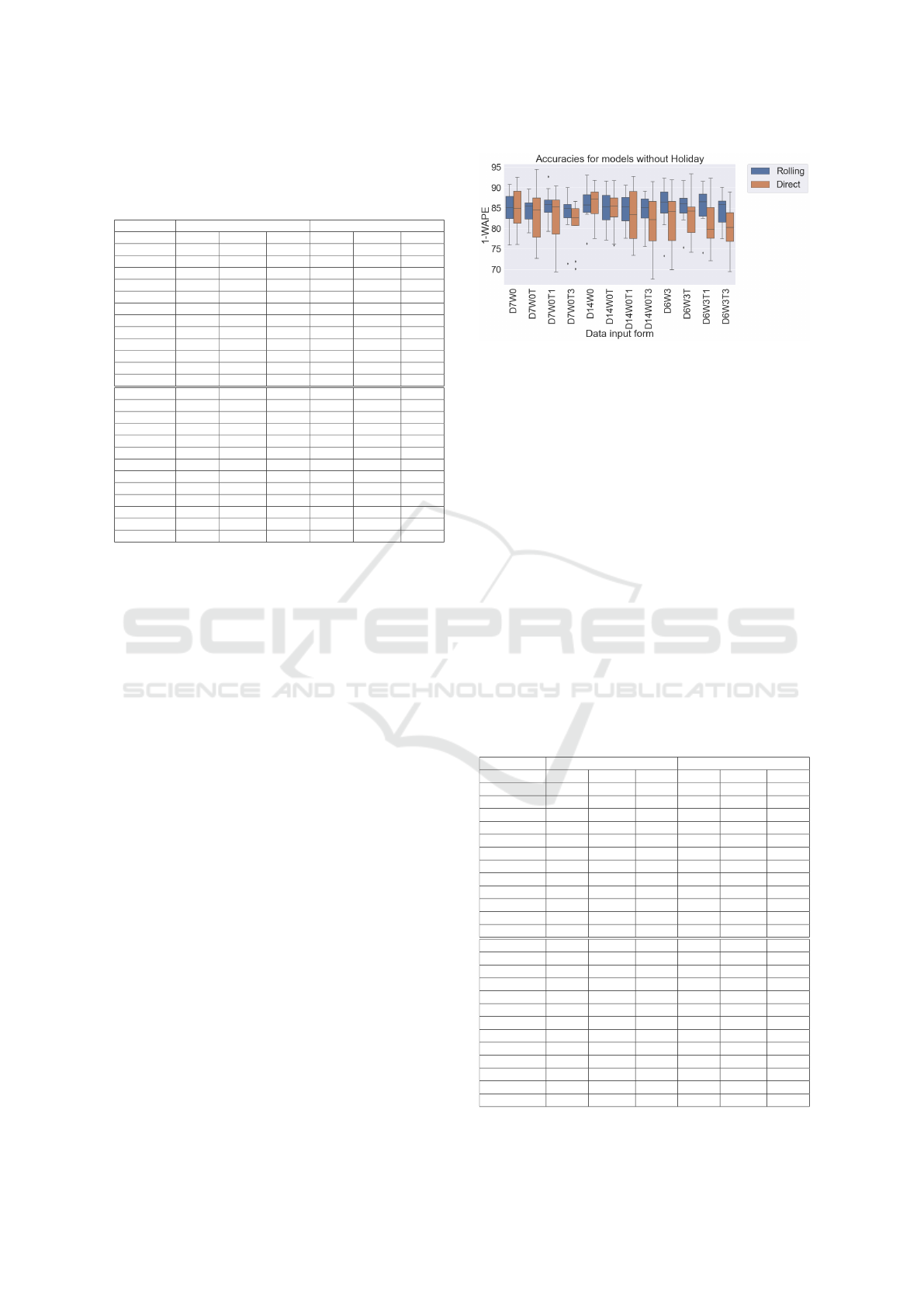
Table 4: 1-WAPE results for the different parking hub mod-

els using DMS and RMS without a holiday input and using

the basic forms with a temperature lag input of 1 and a tem-

perature lag input of 3.

RMS DMS

Form D7W0T1 D14W0T1 D6W3T1 D7W0T1 D14W0T1 D6W3T1

Parking hub1 86.27 88.99 87.24 90.35 89.77 86.31

Parking hub2 86.9 83.07 87.38 84.82 88.23 92.29

Parking hub3 86.97 87.13 85.87 85.74 85.52 77.06

Parking hub4 79.32 78.43 74.09 69.37 73.42 80.33

Parking hub5 82.93 77.59 83.56 73.97 76.44 72.09

Parking hub6 83.87 81.5 82.48 77.78 75.82 75.26

Parking hub7 92.69 90.6 91.49 86.12 80.76 79.24

Parking hub8 89.75 87.69 89.32 89.24 89.39 85.37

Parking hub9 85.44 86.29 88.77 87.21 81.32 84.46

Parking hub10 84 84.35 82.79 80.99 92.72 79.24

Average 85.81 84.56 85.3 82.56 83.34 81.16

Stdev 3.51 4.16 4.67 6.54 6.39 5.67

Form D7W0T3 D14W0T3 D6W3T3 D7W0T3 D14W0T3 D6W3T3

Parking hub1 85.27 86.95 85.94 86.61 83.53 85.24

Parking hub2 84.96 83.73 86.88 80.81 91.46 88.93

Parking hub3 86.1 88.39 85.87 86.34 86.88 83.7

Parking hub4 71.43 79.85 77.49 71.98 69.36 76.42

Parking hub5 81 75.56 81.1 70.13 67.61 78.71

Parking hub6 82.43 82.31 82.93 84.96 78.03 73.48

Parking hub7 90 89.13 90.07 81.91 80.8 78.22

Parking hub8 89.31 87.29 88.28 84.62 85.86 83.91

Parking hub9 84.76 86.41 86.02 83.51 76.62 81.78

Parking hub10 83.23 83.18 81 80.7 88.68 69.47

Average 83.85 84.28 84.56 81.16 80.88 79.99

Stdev 4.91 4.03 3.64 5.43 7.59 5.57

D6W3 with a target day temperature input (D6W3T),

the accuracy raised by around 1%.

From a different view, the parking hub level re-

sults reveal some interesting behavior. Parking hub 1

achieved the best accuracy with the form D7W0 us-

ing the DMS with an accuracy difference of 5% to

the D7W0 with RMS and 3.5% difference with the

best RMS basic form D14W0 for station 1. Addition-

ally, the temperature of the target day increased the

accuracy to around 94.5% which is a further improve-

ment. Parking hub 2 produced the best accuracy with

the RMS when D6W3 form was used (5% better than

D7W0), yet achieved 1% better performance when

D14W0 and D6W3 were used by the DMS. In the

case of the input form D7W0 in parking hubs 4 and

5, the accuracy was raised by around 3% by adding

the temperature of the target day. In parking hub 10,

the best demand prediction was achieved using the

D14W0 form with the temperature of the target day,

with a signiﬁcant difference in the accuracy of 5%.

These cases indicate the DMS can make a signiﬁcant

impact on the accuracy based on the used data.

Figure 5 shows the distribution of model perfor-

mance over 10 different parking hubs in all the cases

of tables 3 and 4. The interquartile range for the RMS

models is smaller in all the different cases, indicat-

ing more stability in the performance when compared

to the RMS. However, in some cases, and depending

on the data, it was observed that the DMS provides

some advantage. The maximum of the DMS models

for D7W0, D7W0T, D14W0T, D14W0T1, D6W3T,

and D6W3T1 is higher than the RMS models. The

Figure 5: Boxplot for accuracy of the models that did not

considered a holiday input in both the DMS and RMS ap-

proaches.

main issue with the DMS in the case study is the vari-

ance. The standard deviation of the performance pa-

rameter is higher for the DMS models than the RMS

models and this is clearly observed via the Figure 5

and supported by the tables 3 and 4.

In general, the RMS performance was better than

the DMS. However, on the level of the parking hub,

some DMS models improved the predictions signif-

icantly. Moreover, the temperature input did not

increase the accuracy signiﬁcantly except for some

parking hubs which indicates that only some parking

hub booking demands are temperature dependent.

4.2 Model Performance with Additional

Holiday Input

Table 5: 1-WAPE results for the different parking hub mod-

els using DMS and RMS with a holiday input and using the

basic forms and the basic forms with temperature inputs.

RMS DMS

Form D7W0 D14W0 D6W3 D7W0 D14W0 D6W3

Parking hub1 90.62 93.01 94.13 91.72 92.17 92.73

Parking hub2 91.39 90.34 90.77 87.68 93.5 92.4

Parking hub3 86.1 84.54 85.87 83.57 78.76 77.18

Parking hub4 87.24 89.85 73.3 92.08 88.05 84.79

Parking hub5 88.47 88.87 89.71 87.31 88.14 87.35

Parking hub6 92.85 90.49 90.77 91.04 88 88.54

Parking hub7 91.7 93.08 89.61 90.24 95.34 92.84

Parking hub8 95.32 97.02 96.36 94.61 97.24 95.48

Parking hub9 91.85 90.31 90.04 90.38 92.39 91.35

Parking hub10 92.91 94.57 91.7 93.52 95.79 96.01

Average 90.84 91.21 89.23 90.22 90.94 89.87

Stdev 2.68 3.25 5.93 3.1 5.16 5.38

Form D7W0T D14W0T D6W3T D7W0T D14W0T D6W3T

Parking hub1 92.26 93.18 92.38 90.45 90.45 92.42

Parking hub2 91.29 90.35 90.18 85.56 85.56 92.97

Parking hub3 86.17 84.54 85.87 83.57 83.57 70.15

Parking hub4 85.12 89.18 74.09 88.74 88.74 82.55

Parking hub5 90.85 88.05 90.9 90.72 90.72 88.58

Parking hub6 92.66 92 93.84 89.97 89.97 87.06

Parking hub7 89.16 91.19 89.01 88.3 88.3 95.84

Parking hub8 96.15 97.16 95.79 94.99 94.99 91.85

Parking hub9 90.66 90.95 91.8 91.4 91.4 91.03

Parking hub10 90.15 92.58 91.73 91.11 91.11 90.43

Average 90.45 90.92 89.56 89.48 89.48 88.29

Stdev 3 3.17 5.75 3.03 3.03 6.96

NCTA 2022 - 14th International Conference on Neural Computation Theory and Applications

364

Table 6: 1-WAPE results for the different parking hub mod-

els using DMS and RMS with a holiday input and using the

basic forms with a temperature lag input of 1 and a temper-

ature lag input of 3.

RMS DMS

Form D7W0T1 D14W0T1 D6W3T1 D7W0T1 D14W0T1 D6W3T1

Parking hub1 91.34 93.36 91.62 91.13 94.11 93.94

Parking hub2 92.36 89.22 91.23 88.64 90.02 95.65

Parking hub3 86.17 84.54 85.87 83.57 81.96 72.02

Parking hub4 85.84 89.49 74.09 90.17 89.27 78.25

Parking hub5 93.9 87.26 90.85 85.69 90.31 87.86

Parking hub6 96.38 91.97 93.82 89.83 93.77 87.45

Parking hub7 89.9 87.69 87.08 89.22 94.24 95.04

Parking hub8 96.8 97.03 96.55 95.64 95.95 95.37

Parking hub9 91.94 90.74 91.95 89.59 90.45 90.19

Parking hub10 92.6 92.39 91.35 94.56 92.84 91.96

Average 91.72 90.37 89.44 89.8 91.29 88.77

Stdev 3.5 3.36 5.86 3.41 3.76 7.5

Form D7W0T3 D14W0T3 D6W3T3 D7W0T3 D14W0T3 D6W3T3

Parking hub1 93.97 92.05 92.53 93.99 93.05 96.62

Parking hub2 92.47 91.1 93.49 85.89 87.99 87.41

Parking hub3 86.1 84.54 85.87 84.83 79.68 71.6

Parking hub4 89.35 89.9 72.86 91.62 88.79 80.67

Parking hub5 90.16 87.7 91.46 81.54 87.81 88.88

Parking hub6 94.76 92.04 92.63 90.93 92.24 83.55

Parking hub7 91.43 88.44 86.05 80.65 86.22 92.19

Parking hub8 96.08 96.19 96.68 96.39 95.21 93.91

Parking hub9 94.72 93.87 93.55 91.36 90.78 93

Parking hub10 92.56 92.35 91.41 90.79 86.47 86.55

Average 92.16 90.82 89.65 88.8 88.82 87.44

Stdev 2.85 3.15 6.42 5.01 4.15 7.03

The addition of a categorical parameter representing

holiday (i.e, whether the target day is a holiday or a

normal day) made a signiﬁcant improvement to all the

results. Each model’s accuracy was increased by no

less than 5% in comparison to the no holiday input

case. These can be observed in the Tables 5 and 6.

Figure 6: Boxplot for accuracy of the models that consid-

ered a holiday input in both the DMS and RMS approaches.

Also, Figure 6 indicates a huge improvement in

the performance of both the DMS and RMS, in com-

parison to the one in Figure 5. The boxplot shrink-

age and the abrupt improvement in accuracy ampli-

ﬁed the importance of the holiday input for the fore-

cast. Additionally, the variance between the perfor-

mance of the different models decreased in all the

cases. An interesting observation can be seen in the

D6W3 form variants. There is an outlier in each in-

put form that has an accuracy lower than the major-

ity of the other models. When comparing the D6W3

in Figure 5 and Figure 6, the input form is causing

more outlier with lower accuracy than the input form

D14W0 and D7W0.

The analysis of the results indicates that the RMS

with a holiday input had the best performance. Al-

though in some case the DMS was observed to be

better than the RMS, the trade-off between the com-

putational cost and the performance make the RMS

the better strategy as a whole. The possible reason

behind the weakness of the DMS is the unsuitability

of the model and also the lack of previous day signal,

thus not capturing the trend. Moreover, the DMS fa-

vored the simplest data input forms (e.g. D7W0 with

and without a holiday) and was able to outperform the

RMS in only few of the cases when a long sequence of

day lags (D14W0) was provided, indicating the need

for a large number of correlated input to produce su-

perior results for speciﬁc parking hubs.

5 CONCLUSION

In this paper, we make use of a telecommunication

service provider’s data on the use of the ﬂeet of vehi-

cles by its employees to analyze and forecast the ve-

hicle booking demand for the future. For that, a com-

parison of the accuracy results using the DMS against

the RMS is done. It was observed that the RMS per-

formance was superior to the DMS in the majority

of the cases and with a signiﬁcantly lower computa-

tional cost. The holiday inputs were found to improve

the prediction quality by about 5% for both the RMS

and the DMS methods. The results suggest that, for

our problem, the RMS forecasting method is better

suited in comparison to the DMS. Some outliers were

seen in the accuracy of the results such as in park-

ing hub 5, and without any external inputs, where the

DMS showed improved accuracy when compared to

the RMS.

The tested models were built into a tool, which

trains the data with all models and automatically

keeps the one with the highest accuracy for each park-

ing hub. The built tool is being trialed by our partner

telecom and encouraging feedback is being received

on the effect of the better forecast have on the resource

management task.

REFERENCES

Azadeh, S. S., Marcotte, P., and Savard, G. (2015). A non-

parametric approach to demand forecasting in revenue

management. Computers & Operations Research,

63:23–31.

Bakker, M., Van Duist, H., Van Schagen, K., Vreeburg, J.,

and Rietveld, L. (2014). Improving the performance

of water demand forecasting models by using weather

input. Procedia Engineering, 70:93–102.

Investigating Prediction Models for Vehicle Demand in a Service Industry

365

Bouktif, S., Fiaz, A., Ouni, A., and Serhani, M. A.

(2018). Optimal deep learning lstm model for elec-

tric load forecasting using feature selection and ge-

netic algorithm: Comparison with machine learning

approaches. Energies, 11(7):1636.

Chen, T. and Guestrin, C. (2016). Xgboost: A scalable

tree boosting system. In Proceedings of the 22nd

ACM SIGKDD International Conference on Knowl-

edge Discovery and Data Mining, KDD ’16, page

785–794, New York, NY, USA. Association for Com-

puting Machinery.

Deschepper, M., Eeckloo, K., Malfait, S., Benoit, D., Cal-

lens, S., and Vansteelandt, S. (2021). Prediction of

hospital bed capacity during the covid- 19 pandemic.

BMC health services research, 21(1):1–10.

Dineva, A., Csom

os, B., Sz, S. K., and Vajda, I. (2021).

Investigation of the performance of direct forecasting

strategy using machine learning in state-of-charge pre-

diction of li-ion batteries exposed to dynamic loads.

Journal of Energy Storage, 36:102351.

Dossani, A. (2022). Inference in direct multi-step and long

horizon forecasting regressions. Available at SSRN

4020488.

Du, P., Jin, Y., and Zhang, K. (2016). A hybrid multi-step

rolling forecasting model based on ssa and simulated

annealing—adaptive particle swarm optimization for

wind speed. Sustainability, 8(8):754.

Feng, B., Xu, J., Zhang, Y., and Lin, Y. (2021). Multi-

step trafﬁc speed prediction based on ensemble learn-

ing on an urban road network. Applied Sciences,

11(10):4423.

Friedman, J. H. (2001). Greedy function approximation: a

gradient boosting machine. Annals of statistics, pages

1189–1232.

Geurts, P., Ernst, D., and Wehenkel, L. (2006). Extremely

randomized trees. Machine learning, 63(1):3–42.

Goic, M., Bozanic-Leal, M. S., Badal, M., and Basso, L. J.

(2021). Covid-19: Short-term forecast of icu beds in

times of crisis. Plos one, 16(1):e0245272.

Herrer

ıa-Alonso, S., Su

arez-Gonz

alez, A., Rodr

ıguez-

erez, M., Rodr

ıguez-Rubio, R. F., and L

opez-

Garc

ıa, C. (2021). Efﬁcient wind speed forecast-

ing for resource-constrained sensor devices. Sensors,

21(3):983.

Hornik, K., Stinchcombe, M., and White, H. (1989). Multi-

layer feedforward networks are universal approxima-

tors. Neural networks, 2(5):359–366.

James, G., Witten, D., Hastie, T., and Tibshirani, R. (2021).

Statistical Learning, pages 15–57. Springer US, New

York, NY.

Ke, G., Meng, Q., Finley, T., Wang, T., Chen, W., Ma, W.,

Ye, Q., and Liu, T.-Y. (2017). Lightgbm: A highly

efﬁcient gradient boosting decision tree. Advances in

neural information processing systems, 30.

Khalid, M. (2019). Wind power economic dispatch–impact

of radial basis functional networks and battery energy

storage. IEEE Access, 7:36819–36832.

Lee, M. (2018). Modeling and forecasting hotel room de-

mand based on advance booking information. Tourism

Management, 66:62–71.

Liu, D., Lu, J., and Ma, W. (2021a). Real-time return de-

mand prediction based on multisource data of one-

way carsharing systems. Journal of Advanced Trans-

portation, 2021.

Liu, Y., Wang, H., Feng, W., and Huang, H. (2021b). Short

term real-time rolling forecast of urban river water

levels based on lstm: A case study in fuzhou city,

china. International Journal of Environmental Re-

search and Public Health, 18(17):9287.

Mu, B., Peng, C., Yuan, S., and Chen, L. (2019). Enso

forecasting over multiple time horizons using convl-

stm network and rolling mechanism. In 2019 inter-

national joint conference on neural networks (ijcnn),

pages 1–8. IEEE.

uller, J. and Bogenberger, K. (2015). Time series analysis

of booking data of a free-ﬂoating carsharing system

in berlin. Transportation Research Procedia, 10:345–

354.

Shi, X. and Yeung, D.-Y. (2018). Machine learning for spa-

tiotemporal sequence forecasting: A survey. arXiv

preprint arXiv:1808.06865.

Sun, S., Wu, H., and Xiang, L. (2020). City-wide traf-

ﬁc ﬂow forecasting using a deep convolutional neural

network. Sensors, 20(2):421.

Surakhi, O., Zaidan, M. A., Fung, P. L., Hossein Motlagh,

N., Serhan, S., AlKhanafseh, M., Ghoniem, R. M.,

and Hussein, T. (2021). Time-lag selection for time-

series forecasting using neural network and heuristic

algorithm. Electronics, 10(20):2518.

Taieb, S. B., Bontempi, G., Atiya, A. F., and Sorjamaa, A.

(2012). A review and comparison of strategies for

multi-step ahead time series forecasting based on the

nn5 forecasting competition. Expert systems with ap-

plications, 39(8):7067–7083.

Vassallo, D., Krishnamurthy, R., Sherman, T., and Fer-

nando, H. J. (2020). Analysis of random forest mod-

eling strategies for multi-step wind speed forecasting.

Energies, 13(20):5488.

Wang, C.-C., Chien, C.-H., and Trappey, A. J. (2021a). On

the application of arima and lstm to predict order de-

mand based on short lead time and on-time delivery

requirements. Processes, 9(7):1157.

Wang, Y., Zhang, N., and Chen, X. (2021b). A short-term

residential load forecasting model based on lstm re-

current neural network considering weather features.

Energies, 14(10):2737.

Yu, D., Li, Z., Zhong, Q., Ai, Y., and Chen, W. (2020). De-

mand management of station-based car sharing sys-

tem based on deep learning forecasting. Journal of

Advanced Transportation, 2020.

Yuan, S., Luo, X., Mu, B., Li, J., and Dai, G. (2019). Pre-

diction of north atlantic oscillation index with convo-

lutional lstm based on ensemble empirical mode de-

composition. Atmosphere, 10(5):252.

Yuan, S., Wang, C., Mu, B., Zhou, F., and Duan, W. (2021).

Typhoon intensity forecasting based on lstm using the

rolling forecast method. Algorithms, 14(3):83.

Zou, H. and Hastie, T. (2003). Regression shrinkage and

selection via the elastic net, with applications to mi-

croarrays. JR Stat Soc Ser B, 67:301–20.

NCTA 2022 - 14th International Conference on Neural Computation Theory and Applications

366