An Improved Support Vector Model with Recursive Feature Elimination
for Crime Prediction
Sphamandla I. May
∗
, Omowunmi E. Isafiade and Olasupo O. Ajayi
Department of Computer Science, University of the Western Cape, Bellville, Cape Town, 7535, South Africa
∗
fi
Keywords:
Crime Prediction, Support Vector Machine, Recursive Feature Elimination, Feature Selection.
Abstract:
The Support Vector Machine (SVM) model has proven relevant in several applications, including crime analy-
sis and prediction. This work utilized the SVM model and developed a predictive model for crime occurrence
types. The SVM model was then enhanced using feature selection mechanism, and the enhanced model was
compared to the classical SVM. To evaluate the classical and enhanced models, two distinct datasets, one from
Chicago and the other from Los Angeles, were used for experiment. In an attempt to enhance the performance
of the SVM model and reduce complexity, this work utilised relevant feature selection techniques. We used
the Recursive Feature Elimination (RFE) model to enhance SVM’s performance and reduce its complexity,
and observed performance increase of an average of 15% from the City of Chicago dataset and 20% from
the Los Angeles dataset. Thus, incorporation of appropriate feature selection techniques enhances predictive
power of classification algorithms.
1 INTRODUCTION
Recent statistics have shown that crime rates have
been on the increase annually, with an exponen-
tial increase in the last few decades (Ceccato and
Loukaitou-Sideris, 2022). This increase in crime rate
poses a serious threat to the stability of societies, in-
cluding financial and psycho-physiological (such as
Post Traumatic Stress Disorder) effect on citizenry
(Kushner et al., 1993). This continuous increase in
crime rates can be an indicative parameter to exam-
ine the capabilities and/or limitations of current crime
preventative strategies. Fortunately, the last few years
have witnessed an increase in crime scene monitor-
ing systems, specifically for reporting and investiga-
tive purposes. Crime records can then be analysed and
used to develop preventative strategies for crime pre-
diction. However, due to the large number of crimes,
associated crime records are voluminous and gathered
at a fast rate, making manual processing and analysis
ineffective. Thus, intelligent means of analysis such
as the use of machine learning is inevitable.
Machine learning has been extensively used in
crime prediction and able to successfully anticipate
the occurrence of crime, the possible location, as well
as the type of crime that might occur (Kim et al.,
2018),(Lin et al., 2018), (Alves et al., 2018), (Bogo-
molov et al., 2014), and (Chun et al., 2019). With
this ability, law enforcement personnel and agencies
can strategise and effectively allocate scarce resource
to improve service delivery. There are a variety of
machine learning algorithms that are used in crime,
such as the Decision Tree, Random Forests, Extra
Trees (May et al., 2021b), Deep learning, Support
Vector Machines (SVM)(Cao and Chong, 2002). In
this study, SVM is used to predict potential crime
type. This work also attempts to improve the perfor-
mance of the classic SVM algorithm for crime pre-
diction by combining it with Recursive Feature Elim-
ination (RFE) approach, similar to what was done in
(May et al., 2021a). To the best of the researchers’
knowledge, there is no research that has considered
enhancing the SVM model for crime analysis using
this approach.
2 LITERATURE REVIEW
There are various research on crime analysis and
prediction, with numerous methodologies and theo-
ries used to attain the common objective of predict-
ing crime and implementing preventive actions (Lin
et al., 2018), (Sivaranjani et al., 2016), (Islam and
Raza, 2020),(Isafiade and Bagula, 2020), (Kiran and
Kaishveen, 2018). A variety of machine learning al-
gorithms, which can be broadly classed as regression,
196
May, S., Isafiade, O. and Ajayi, O.
An Improved Support Vector Model with Recursive Feature Elimination for Crime Prediction.
DOI: 10.5220/0011524200003335
In Proceedings of the 14th International Joint Conference on Knowledge Discovery, Knowledge Engineering and Knowledge Management (IC3K 2022) - Volume 1: KDIR, pages 196-203
ISBN: 978-989-758-614-9; ISSN: 2184-3228
Copyright
c
 2022 by SCITEPRESS – Science and Technology Publications, Lda. All rights reserved

clustering, and classification, have been applied to
crime analysis.
Clustering models, in addition to the ARIMA
model, have been effectively used in the construction
of robust predictive models, as shown in (Sivaran-
jani et al., 2016), (Kiran and Kaishveen, 2018), (Ro-
driguez et al., 2017), and (Hajela et al., 2020). The au-
thors in (Hajela et al., 2020) used k-means to improve
the predictive power of different classification algo-
rithms, such as Nave Bayes, Decision Trees, and en-
semble learning approaches. Obtained results showed
that the incorporation of k-means clustering method
improved the classification accuracies of the base al-
gorithms.
While clustering enhanced models have been
shown to improve classification accuracies, most re-
searchers still rely on manual feature selection meth-
ods. It has also been reported that feature selection
can increase a model’s accuracy and in some cases
decrease the complexity (Chu et al., 2012). How-
ever, despite this, the vast majority of scholars that
investigated crime prediction via the lens of classi-
fication, such as (Hajela et al., 2020), (Ivan et al.,
2017a), (Zaidi et al., 2019), (Iqbal et al., 2013), and
(Ivan et al., 2017b), did not adopt feature selection
approaches. There are several feature selection strate-
gies, including intrinsic (or embedded), regulariza-
tion, filter, and wrapper strategies. The intrinsic tech-
niques allude to the algorithm’s capacity to execute
feature selection on its own. Tree-based algorithms,
such as Decision Trees, Random Forests, and Ex-
tremely Randomized Trees are all capable of perform-
ing feature selection on their own; hence, can be con-
sidered intrinsic (May et al., 2021b), (Sylvester et al.,
2018).
Other than the tree-based algorithms, there are
also regularization methods which utilize a form of
intrinsic penalization function to reduce over-fitting.
Examples of these techniques are the Least Absolute
Shrinkage and Selection Operator (LASSO) that per-
forms L1 regularization (Baraniuk, 2007) and Ridge
Regression that performs L2 regularization (Hilt and
Seegrist, 1977). In (Nitta et al., 2019), the LASSO
feature selection strategy was used to choose the op-
timal subset of features for building a Naive Bayes
and SVM classifier for crime prediction and catego-
rization. Filtering strategies are based on statistics
and the relevance of features. Linear Discriminant
Analysis (LDA), Analysis of Variance (ANOVA), and
Chi-Square are common examples of statistical ap-
proaches. For example, in (Mohd et al., 2017), the
correlation feature evaluator, correlation-based fea-
ture subset evaluator, and information gain were in-
vestigated as three different forms of filter selection
techniques. These three strategies were used to de-
termine the optimal collection of features required
to build a crime prediction classifier. The authors
concluded that the combination of correlation feature
evaluator and correlation-based feature subset evalua-
tor was the best feature selection approach, after eval-
uating their methods on a community crime dataset.
Wrapper feature selection methods search for the
best performing subset of features. These wrapper
strategies initially pick a subset of features to be
used in training given models, then iteratively adds
or removes features from the subset based on the in-
ferences returned. The wrapper category includes
several techniques, with the most noteworthy being
the Forward Selection, Backward Selection, and Re-
cursive Feature Elimination (RFE). Forward feature
selection is an iterative procedure that begins with
no features and incrementally adds them until the
model’s performance is no longer improved. Back-
ward feature selection, in contrast to forward feature
selection, starts with all features and repeatedly re-
moves features until the model’s performance does
not improve. The authors in (Aldossari et al., 2020)
obtained the optimal subset of features to train a De-
cision Tree and a Nave Bayes classifier for crime
prediction using the backward feature selection tech-
nique. RFE is a form of backward feature selection
method, that scores each feature based on its con-
tribution to the model’s overall performance (Guyon
et al., 2002). The most widely utilized scoring fac-
tor is the feature importance. RFE thus recursively
eliminates least scoring features based on computed
priority or importance. In (Zhu et al., 2018), RFE was
used to choose the best features, which were then fed
into both the Linear Regression and Random Forest
algorithms. RFE was also used in (Kadar et al., 2016)
to create a model for estimating crime counts using
the New York foursquare dataset. In another work,
RFE was combined with Naive Bayes in (May et al.,
2021a) to choose the optimal number of features for
crime prediction. The developed model, which was
tested using the Chicago Citizen Law Enforcement
Analysis and Reporting (CLEAR) dataset, showed a
30% improvement over the pure Naive Bayes model.
In this work, we propose the enhancement of
SVM by combining it with a feature selection model.
This is similar to the work done in (Cao and Chong,
2002) where three component analysis models, Prin-
cipal Component Analysis (PCA), kernel principal
component analysis (KPCA) and independent com-
ponent analysis (ICA) were used with SVM. Unlike
in that work, we apply RFE to perform feature selec-
tion for SVM, then compare this improved SVM to
the pure SVM.
An Improved Support Vector Model with Recursive Feature Elimination for Crime Prediction
197

(a) Two class linearly separable data
(b) Non-linearly separable data
Figure 1: Data separation by Hyperplanes.
3 MODELS AND
EXPERIMENTAL DESIGN
3.1 Support Vector Machine (SVM)
Model
SVM is a non-liner solver for classification and
regression problems developed by Vapnik (Vapnik,
1999). SVM is a widely used ML model be-
cause it can perform both regression and classifica-
tion, works well with small datasets and robustness
against outliers (Mart
´
ınez-Ram
´
on and Christodoulou,
2005),(Wang, 2005). SVM seeks to draw a line (hy-
perplane) to separate data into respective classes, as
illustrated in Fig 1a and 1b.
Formally, the hyperplane in a n-dimensional space
is an n-1 dimensional subspace. For instance, in a two
dimensional space, the hyperplane is a one dimen-
sional straight line. For a set of n training samples,
x
i
,(i = 1,2,. . . ,n), the optimal hyperplane is defined
as shown in Equation (1):
w
T
x + b
(
≤ 1 f or y
i
= 1
≤ −1 f or y
i
= −1
(1)
Where w
T
is the transpose of the n-dimensional
normal vector and b a bias term. Data that lies closest
to the optimal hyperplane either from the right or from
the left are referred to as the support vectors.
This hyperplane must maximise the distance from
support vectors of each class, and must have the
smallest possible data separation error (Steinwart and
Christmann, 2008). Hence, data falls on either of two
sides of the optimal hyper-plane, the left (y = 1) or
right (y = −1). There are instances where the data
sample are not linearly separable, thus not possible to
draw a straight hyperplane. In such instances, a soft
Table 1: Various Kernel functions frequently used for non-
linear data classifications.
Type of Classifier Kernel Function
Sigmoid K(x
i
,x
j
) = (α(x
i
· x
i
) + ϑ)
Multilayer perceptron K(x
i
,x
j
) = tanh(yx
T
i
x
j
+ µ)
Linear K(x
i
,x
j
) = (x
T
i
x
j
)
ρ
Guassian RBF K(x
i
,x
j
) = exp(
−[∥x
i
−x
j
∥
2
]
2υ
2
)
Dirichlet
sin(
n+1
2
)(x
i
−x
j
)
2sin((x
i
−x
j
)/2)
margin is used instead, which can be obtained using
Equation (2):
d(x) =
N
∑
i=1
α
i
y
i
K(x, x
i
) + b (2)
where α
i
is the Lagrange multiplier, b is the bias, and
K is the Kernel function.
The Kernel function (K) is used to separate non-
linearly separable data, by changing into a higher di-
mensional space, where they become linearly separa-
ble. There are several types of kernel functions and
these are summarized in Table 1
3.2 Recursive Feature Elimination
(RFE) Method
As discussed in the literature review section, the RFE
method is a backward approach of selecting features.
It uses models to fill all the features and recursively
eliminates features which either decreases or have no
influence on the overall performance of the selected
model. In this work, the baseline models considered
for the RFE were Linear Regression (LR), Extremely
Randomized Trees (ERT) and Random Forest (RF),
from which the one with the highest accuracy was se-
lected. Fig.2 is a flowchart depicting our process of
integrating RFE into SVM for optimal feature selec-
tion and improved classification.
3.3 Experimental Setup
We conducted our experiment on a Dell Desktop PC
with Intel Core i5 10
th
Gen processor, with a 1.19
GHz base clock, and 8 GB of RAM. Data process-
ing and exploration, coding and evaluation of the
predictive models were all done using Python and
Jupyter Notebook. Furthermore, we used 10 fold
cross-validation to evaluate the models.
3.4 Data Description and
Pre-processing
Two datasets were used to test the models, which are:
i) the Chicago Police Department’s Citizen Law En-
forcement Analysis and Reporting (CLEAR) dataset
KDIR 2022 - 14th International Conference on Knowledge Discovery and Information Retrieval
198

Figure 2: Process of integrating RFE with SVM.
which contains about 7.26 million records of crime
data with 21 features collected between year 2001-
2020 (Cit, 2001a); ii) Los Angeles Dataset, with 2.12
million crime records, and 24 features collected be-
tween year 2010 and 2019 (Cit, 2001b). The CLEAR
dataset initially had 32 unique crimes, from which
we selected the 5 frequently (about 70%) occurring
crimes (about 70% of the entire dataset. These were
Theft, Battery, Criminal Damage, Narcotics, and As-
sault. Similarly, the Los Angeles dataset was filtered
from 110 unique crimes to the top 5 common crimes,
namely Robbery, Battery (Simple Assault), Assault
With Deadly Weapon, Aggravated Assault, Intimate
Partner - Simple Assault. All five were numerically
encoded as 0 to 4. Furthermore, certain features that
we identified as not having high predictive power such
as ID and X, Y coordinates were removed. To this
end, the features left in the CLEAR dataset were: De-
scription, IUCR, FBI Code, Arrest, Longitude, Com-
munity Area, Block, Beat, District, Location Descrip-
tion, Ward, Year, Case Number, Domestic, Updated
On, Latitude, Day, Month, Hour, DayOfWeek, and
WeekOfYear features, for a total of 21 features as
summarized in Table 2. Similar processes were car-
ried out on the Los Angeles dataset, with the final fea-
ture set summarized in Table 3.
3.5 Evaluation Metrics
Accuracy, Precision (P), Recall (R), and F1
Score
were
used to assess the performance of the models. Accu-
Table 2: Features considered in the Chicago Dataset.
Feature Description
Description The secondary description of the IUCR code, a subcategory of
the primary description
IUCR The Illinois Unifrom Crime Reporting code
FBI Code Indicates the crime classification as outlined in the FBI’s FBI
National Incident-Based Reporting System (NIBRS).
Arrest Indicates if an arrest was made
Longitude The longitude of the location where the incident occurred
Latitude The latitude of the location where the incident occurred
Community Area Indicates the community area where the incident occurred
Block Partially redacted address where the incident occurred
but within the same block as the actual address
Beat Indicates the beat where the incident occurred.
A beat is the smallest police geographic area
District Indicates the police district where the incident occurred
Location Description Description of the location where the incident occurred
Ward The ward (City Council district) where the incident occurred
Year Year the incident occurred
Case Number The Chicago Police Department RD Number
(Records Division Number), which is unique to the incident
Domestic Indicates whether the incident was domestic-related as
defined by the Illinois Domestic Violence Act
Updated On Date and time the record was last updated
Month The month the incident occurred
Day The day the incident occurred
DayOfWeek The day of the week the incident occurred
WeekOfYear The week of year the incident occurred
Hour The hour of the day the incident occurred
Table 3: Features considered in the Los Angeles Dataset.
Feature Description
Weapon Used The type of weapon used in the crime
Weapon Desc Defines the Weapon Used Code provided.
Vict Sex Victim Sex, F - Female, M - Male, X - Unknown
Vict Age Two character numeric.
Mocodes Modus Operandi: Activities associated with the suspect
in commission of the crime.
LON The longitude of the location where the incident occurred
LAT The latitude of the location where the incident occurred
Vict Descent Descent Code: A - Other Asian, B - Black, C - Chinese
D- Cambodian, F - Filipino, G - Guamanian ,H - Hispanic/Latin/Mexican
I - American Indian/Alaskan Native, J - Japanese, K - Korean, L - Laotian
O - Other P - Pacific Islander S - Samoan U - Hawaiian V - Vietnamese
W - White X - Unknown Z - Asian Indian
LOCATION Street address of crime incident rounded to the nearest
hundred block to maintain anonymity.
Date Rptd Date Reported, MM/DD/YYYY
AREA NAME The 21 Geographic Areas or Patrol Divisions are also given a name
designation that references a landmark or the surrounding community that it is
responsible for. For example 77th Street Division is located at the intersection
of South Broadway and 77th Street, serving neighborhoods in South Los Angeles.
Premis Cd The type of structure, vehicle, or location where the crime took place.
Premis Desc Defines the Premise Code provided
Status Desc Defines the Status Code provided
Status Status of the case. (IC is the default)
Cross Street Cross Street of rounded Address
Month The month the incident occurred
Day The day the incident occurred
DayOfWeek The day of the week the incident occurred
WeekOfYear The week of year the incident occurred
Hour The hour of the day the incident occurred
TIME OCC The hour of the day the incident occurred
Rpt Dist No A four-digit code that represents a sub-area
within a Geographic Area. All crime records reference the
”RD” that it occurred in for statistical comparisons
racy is a measure of how often the model correctly
classified instances. Precision is the fraction of rel-
evant instances among the successfully retrieved in-
stances, while recall is the fraction of relevant in-
stances that were successfully retrieved. F1
Score
is
obtained from precision and recall by computing their
harmonic mean.
4 RESULTS AND DISCUSSION
As stated earlier, two distinct datasets were used - the
Chicago and Los Angeles dataset. In both datasets
we followed the same procedure of experimentation,
we first varied the C and Gamma values and then
An Improved Support Vector Model with Recursive Feature Elimination for Crime Prediction
199

Table 4: Comparison of Kernel functions on the Chicago
dataset.
Linear Kernel
Evaluation
Metric (%)
Gamma=0.01,
C=0.01
Gamma=1,
C=1
Gamma=10,
C=10
Accuracy 35.80 40.34 55.78
Precision 28.82 47.9 53.79
Recall 35.80 48.01 55.57
F1 Score 27.88 46.8 54.51
Polynomial Kernel
Accuracy 49.34 56.1 65.73
Precision 47.57 54.54 62.56
Recall 46.86 55.36 63.2
F1 Score 45.61 54.54 64.78
Gaussian RBF kernel
Accuracy 59.27 65.9 74.73
Precision 57.45 64.9 71.56
Recall 55.60 66.6 74.2
F1 Score 56.71 63.57 73.78
used three distinct kernels. Gamma value dictates
the radius of influence for single samples, while C is
the trade off between maximization of the decision
function’s margin and correct classification of sam-
ples. Grid Search was used for hyper-parameter tun-
ing (Bergstra and Bengio, 2012). For brevity, we only
show the results for values of 0.01, 1 and 10. Due
to the dataset being non-linearly separable, we used
Kernel functions for feature space transformation. We
considered the Linear, Polynomial, and RBF kernel
functions, in order to determine which of these will
yield a better result (Wang, 2005).
4.1 Performance Comparison of the
Kernel Functions
Table 4 summarizes results obtained from the
Chicago dataset, while Table 5 presents those of the
Los Angeles dataset, based on the different parame-
ters considered.
For the Chicago dataset, it was observed that gen-
erally, the model improved as the parameter values
increased, with the Gaussian RBF kernel having the
best result, followed by Polynomial and Linear ker-
nels.
The results obtained for the Los Angeles dataset
were consistent with those of the Chicago dataset with
similar findings. Observing the different values from
0.01 to 10 for C and Gamma, a gradual performance
increase was noted and the best performance was ob-
tained at 10 as seen on Tables 4 and 5.
4.2 Process of Enhancing SVM with
RFE (RFE-SVM)
This section presents the results obtained by enhanc-
ing the SVM algorithm with RFE as earlier discussed
Table 5: Comparison of Kernel functions on the Los Ange-
les dataset.
Linear Kernel
Evaluation
Metric (%)
Gamma=0.01,
C=0.01
Gamma=1,
C=1
Gamma=10,
C=10
Accuracy 36.61 42.19 56.91
Precision 29.19 48.17 55.78
Recall 36.89 41.19 57.20
F1 Score 28.11 48.1 56.15
Polynomial Kernel
Accuracy 41.52 56.17 6.71
Precision 48.59 56.71 63.19
Recall 44.17 57.61 65.18
F1 Score 45.71 54.81 64.51
Gaussian RBF kernel
Accuracy 59.34 66.1 75.73
Precision 56.51 65.16 73.16
Recall 57.81 64.16 74.58
F1 Score 56.51 65.34 75.51
Table 6: RFE with three (3) models.
Chicago Dataset Los Angeles Dataset
Models Accuracy (%) Accuracy (%)
LR 40.39 39.55
ERT 83.71 82.23
RF 96.33 92.51
and presented in Fig 2.
A. Selecting the RFE Wrapper Model
As discussed earlier, RFE requires a base model
to execute the feature selection process. We con-
sidered three models for this task, which are LR,
ERT, and RF. Table 6 shows a comparison of the
three selected models on the Chicago dataset.
It can be observed that RF outperforms the two
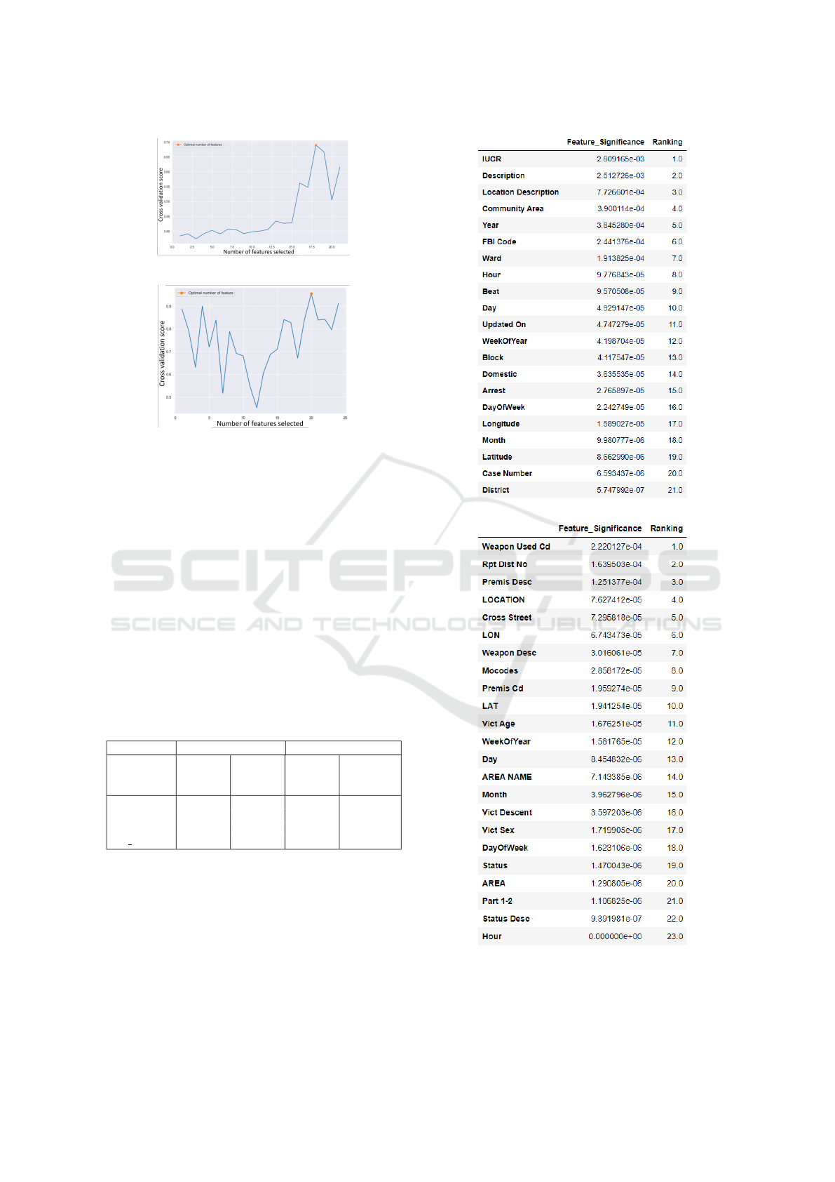
other models, hence it was selected as the wrapper
method to obtain the optimal features as shown in
Fig. 3. The orange dot depicts the peak of the
curve and represent the optimal number of fea-
tures considered. For the Chicago (see Fig. 4a )
and Los Angeles datasets (see Fig. 4b), 21 and
23 features were considered respectively. Fig.
4 presents the list of selected features for both
datasets and ranked by feature importance in a de-
scending order.
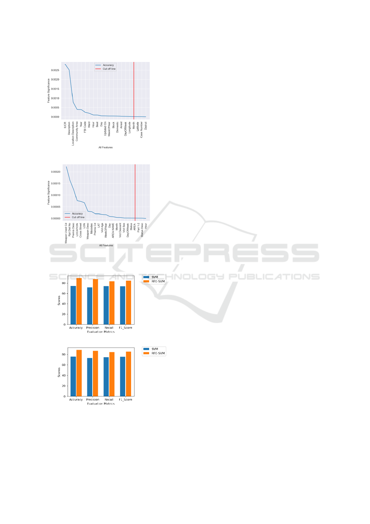
Fig.5 (best viewed in colour mode) presents a line
graph of all feature versus feature significance.
For the Chicago dataset, 18 features were even-
tually selected by the RFE model, thus eliminat-
ing features after the 18 cut-off mark, i.e., the red
vertical line in Fig.5a. For the Chicago dataset,
Latitude, Case Number, and District were deemed
least influential by the wrapper method. A simi-
lar process was carried out for the Los Angeles
dataset, with Part 1-2, Status Desc, and Hour be-
ing the least influential features that were elimi-
nated (see Fig.5b). Thus, 20 features were even-
KDIR 2022 - 14th International Conference on Knowledge Discovery and Information Retrieval
200

(a) Chicago Dataset
(b) Los Angeles Dataset
Figure 3: Optimal number of features selected by RFE for
both Chicago and Los Angeles datasets.
tually selected by the feature selection model.
B. Enhanced SVM (RFE-SVM)
Having identified the most significant features,
we ran two simulations with SVM, the first with
all features (tagged ”Pure SVM”) and the sec-
ond with the RFE selected features (tagged ”RFE-
SVM”). Table 7 shows a comparison of both mod-
els, and reveals that for all the metrics, the en-
hanced version had a 20% performance boost on
the average for Chicago dataset and 15% for the
Los Angeles dataset. Fig. 6 gives a graphical de-
piction of the comparisons.
Table 7: Comparison of Enhanced SVM with Pure SVM.
Chicago Dataset Los Angeles Dataset
Evaluation
Met-
rics(%)
Pure
SVM
RFE-
SVM
Pure
SVM
RFE-
SVM
Accuracy 74.73 89.91 75.73 88.7
Precision 71.56 87.57 73.16 86.96
Recall 74.20 83.41 74.58 84.37
F1 Score 73.78 84.59 75.51 85.33
5 CONCLUSION
There are numerous machine learning (ML) algo-
rithms in use in a wide variety of disciplines includ-
ing finance, medical, crime, to mention a few. Com-
mon among these ML models is the Support Vector
Machine (SVM). This study considered the efficacy
of SVM for crime prediction, and adopted feature
(a) Chicago Dataset
(b) Los Angeles Dataset
Figure 4: Selected features ranked by significance.
An Improved Support Vector Model with Recursive Feature Elimination for Crime Prediction
201

(a) Chicago Dataset
(b) Los Angeles Dataset
Figure 5: Feature significance and cut-off feature.
(a) Chicago Dataset
(b) Los Angeles Dataset
Figure 6: Comparative evaluation of RFE-SVM and SVM.
selection mechanism to enhance the performance of
SVM. Two crime datasets were used, the Chicago Po-
lice department’s Citizen Law Enforcement Analysis
and Reporting system (CLEAR) dataset, and the Los
Angeles crime dataset. In applying SVM, three ker-
nels were compared, Linear, Polynomial and Guas-
sian RBF, with the Guassian RBF proving to be the
best of these kernels based on results obtained. To en-
hance the performance of SVM, this work introduced
the use of feature selection through Recursive Feature
Elimination (RFE). RFE was used to select the opti-
mal number of features from the datasets before ap-
plying SVM (RFE-SVM). We then compared the per-
formance of the classic SVM with the enhanced SVM
(i.e., RFE-SVM model). This enhancement improved
the prediction accuracy of SVM by up to 15% in the
Los Angeles dataset and 20% for the Chicago dataset.
It can therefore be concluded that the incorporation of
feature selection algorithms enhanced SVM’s perfor-
mance.
REFERENCES
(2001a). Crimes - 2001 to present - Dash-
board — City of Chicago — Data Portal.
https://data.cityofchicago.org/Public-Safety/
Crimes-2001-to-present-Dashboard/5cd6-ry5g.
(2001b). Crimes - 2010 to 2019 - Dashboard — Los
Angeles — Data Portal. https://data.lacity.org/
Public-Safety/Crime-Data-from-2010-to-2019/
63jg-8b9z.
Aldossari, B. S., Alqahtani, F. M., Alshahrani, N. S., Al-
hammam, M. M., Alzamanan, R. M., and Aslam, N.
(2020). A comparative study of decision tree and
naive bayes machine learning model for crime cate-
gory prediction in chicago. In Proc. of the 6th Inter-
national Conf. on Computing and Data Engineering,
pages 34–38.
Alves, L. G., Ribeiro, H. V., and Rodrigues, F. A. (2018).
Crime prediction through urban metrics and statisti-
cal learning. Physica A: Statistical Mechanics and its
Applications, 505:435–443.
Baraniuk, R. G. (2007). Compressive sensing [lecture
notes]. IEEE signal processing magazine, 24(4):118–
121.
Bergstra, J. and Bengio, Y. (2012). Random search for
hyper-parameter optimization. J. machine learning re-
search, 13(2).
Bogomolov, A., Lepri, B., Staiano, J., Oliver, N., Pianesi,
F., and Pentland, A. (2014). Once upon a crime: to-
wards crime prediction from demographics and mo-
bile data. In Proc. of the 16th international Conf. on
multimodal interaction, pages 427–434.
Cao, L. and Chong, W. (2002). Feature extraction in support
vector machine: a comparison of pca, xpca and ica.
In Proc. of the 9th International Conf. on Neural In-
formation Processing, 2002. ICONIP ’02., volume 2,
pages 1001–1005.
KDIR 2022 - 14th International Conference on Knowledge Discovery and Information Retrieval
202

Ceccato, V. and Loukaitou-Sideris, A. (2022). Fear of sex-
ual harassment and its impact on safety perceptions in
transit environments: a global perspective. Violence
against women, 28(1):26–48.
Chu, C., Hsu, A.-L., Chou, K.-H., Bandettini, P., Lin, C.,
Initiative, A. D. N., et al. (2012). Does feature selec-
tion improve classification accuracy? impact of sam-
ple size and feature selection on classification using
anatomical magnetic resonance images. Neuroimage,
60(1):59–70.
Chun, S. A., Avinash Paturu, V., Yuan, S., Pathak, R.,
Atluri, V., and R. Adam, N. (2019). Crime predic-
tion model using deep neural networks. In Proc. of
the 20th Annual International Conf. on Digital Gov-
ernment Research, pages 512–514.
Guyon, I., Weston, J., Barnhill, S., and Vapnik, V. (2002).
Gene selection for cancer classification using support
vector machines. Machine learning, 46(1):389–422.
Hajela, G., Chawla, M., and Rasool, A. (2020). A clus-
tering based hotspot identification approach for crime
prediction. Procedia Computer Science, 167:1462–
1470.
Hilt, D. E. and Seegrist, D. W. (1977). Ridge, a computer
program for calculating ridge regression estimates,
volume 236. Department of Agriculture, Forest Ser-
vice, Northeastern Forest Experiment . . . .
Iqbal, R., Murad, M. A. A., Mustapha, A., Panahy, P. H. S.,
and Khanahmadliravi, N. (2013). An experimental
study of classification algorithms for crime prediction.
Indian J. Science and Technology, 6(3):4219–4225.
Isafiade, O. E. and Bagula, A. B. (2020). Series mining for
public safety advancement in emerging smart cities.
Future Generation Computer Systems, 108:777–802.
Islam, K. and Raza, A. (2020). Forecasting crime using
arima model. arXiv preprint arXiv:2003.08006.
Ivan, N., Ahishakiye, E., Omulo, E. O., and Taremwa, D.
(2017a). Crime prediction using decision tree (j48)
classification algorithm.
Ivan, N., Ahishakiye, E., Omulo, E. O., and Wario, R.
(2017b). A performance analysis of business intel-
ligence techniques on crime prediction.
Kadar, C., Iria, J., and Cvijikj, I. P. (2016). Exploring
foursquare-derived features for crime prediction in
new york city. In The 5th international workshop on
urban computing (UrbComp 2016). ACM.
Kim, S., Joshi, P., Kalsi, P. S., and Taheri, P. (2018). Crime
analysis through machine learning. In 2018 IEEE
9th Annual Information Technology, Electronics and
Mobile Communication Conf. (IEMCON), pages 415–
420. IEEE.
Kiran, J. and Kaishveen, K. (2018). Prediction analysis of
crime in india using a hybrid clustering approach. In
2018 2nd International Conf. on I-SMAC (IoT in So-
cial, Mobile, Analytics and Cloud), pages 520–523.
IEEE.
Kushner, M. G., Riggs, D. S., Foa, E. B., and Miller, S. M.
(1993). Perceived controllability and the development
of posttraumatic stress disorder (ptsd) in crime vic-
tims. Behaviour research and therapy, 31(1):105–
110.
Lin, Y.-L., Yen, M.-F., and Yu, L.-C. (2018). Grid-based
crime prediction using geographical features. ISPRS
International J. Geo-Information, 7(8):298.
Mart
´
ınez-Ram
´
on, M. and Christodoulou, C. (2005). Sup-
port vector machines for antenna array processing and
electromagnetics. Synthesis Lectures on Computa-
tional Electromagnetics, 1(1):1–120.
May, S., Isafiade, O., and Ajayi, O. (2021a). An enhanced
na
¨
ıve bayes model for crime prediction using recur-
sive feature elimination. New York, NY, USA. Asso-
ciation for Computing Machinery.
May, S., Isafiade, O., and Ajayi, O. (2021b). Hybridizing
extremely randomized trees with bootstrap aggrega-
tion for crime prediction. New York, NY, USA. Asso-
ciation for Computing Machinery.
Mohd, F., Noor, N. M. M., et al. (2017). A comparative
study to evaluate filtering methods for crime data fea-
ture selection. Procedia computer science, 116:113–
120.
Nitta, G. R., Rao, B. Y., Sravani, T., Ramakrishiah, N., and
Balaanand, M. (2019). Lasso-based feature selection
and na
¨
ıve bayes classifier for crime prediction and its
type. Service Oriented Computing and Applications,
13(3):187–197.
Rodriguez, C. D. R., Gomez, D. M., and Rey, M. A. M.
(2017). Forecasting time series from clustering by a
memetic differential fuzzy approach: An application
to crime prediction. In 2017 IEEE Symposium Se-
ries on Computational Intelligence (SSCI), pages 1–8.
IEEE.
Sivaranjani, S., Sivakumari, S., and Aasha, M. (2016).
Crime prediction and forecasting in tamilnadu using
clustering approaches. In 2016 International Conf. on
Emerging Technological Trends (ICETT), pages 1–6.
IEEE.
Steinwart, I. and Christmann, A. (2008). Support vector
machines. Springer Science & Business Media.
Sylvester, E. V. A., Bentzen, P., Bradbury, I. R., Cl
´
ement,
M., Pearce, J., Horne, J., and Beiko, R. G. (2018).
Applications of random forest feature selection for
fine-scale genetic population assignment. Evolution-
ary Applications, 11(2):153–165.
Vapnik, V. N. (1999). An overview of statistical learning
theory, volume 10. IEEE.
Wang, L. (2005). Support vector machines: theory and ap-
plications, volume 177. Springer Science & Business
Media.
Zaidi, N. A. S., Mustapha, A., Mostafa, S. A., and Razali,
M. N. (2019). A classification approach for crime pre-
diction. In International Conf. on Applied Comput-
ing to Support Industry: Innovation and Technology,
pages 68–78. Springer.
Zhu, Y. et al. (2018). Comparison of model perfor-
mance for basic and advanced modeling approaches
to crime prediction. Intelligent Information Manage-
ment, 10(06):123.
An Improved Support Vector Model with Recursive Feature Elimination for Crime Prediction
203