Par-VSOM: Parallel and Stochastic Self-organizing Map Training

Algorithm

Omar X. Rivera-Morales and Lutz Hamel

Department of Computer Science, University of Rhode Island, College Road, South Kingstown, Rhode Island, U.S.A.

Keywords:

SOM, VSOM, GPU, Parallel Computing, Self-organizing Map, Stochastic Training, Vector Optimization.

Abstract:

This work proposes Par-VSOM, a novel parallel version of VSOM, a very efﬁcient implementation of stochas-

tic training for self-organizing maps inspired by ideas from tensor algebra. The new algorithm is implemented

using parallel kernels on GPU accelerators. It provides performance increases over the original VSOM algo-

rithm, PyTorch Quicksom parallel version, Tensorﬂow Xpysom parallel variant, as well as Kohonen’s classic

iterative implementation. Here we develop the algorithm in some detail and then demonstrate its performance

on several real-world datasets. We also demonstrate that our new algorithm does not sacriﬁce map quality for

speed using the convergence index quality assessment.

1 INTRODUCTION

The self-organizing map (SOM) is a neural network

designed for unsupervised machine learning (Koho-

nen, 2001). The generated maps are powerful data

analysis tools applied to diverse areas such as atmo-

spheric science, nuclear physics, pattern recognition,

medical diagnosis, computer vision and other data do-

mains (Barney, 2018; Li et al., 2018a; Ramos et al.,

2017). See reference (Kohonen, 2001) for a more

comprehensive literature survey. Here we introduce

the Parallel VSOM (Par-VSOM), a parallel imple-

mentation of the efﬁcient VSOM algorithm (Hamel,

2019). The novel approach presented here, replaces

all iterative constructs of the SOM algorithm with

kernels running in a hardware accelerator to perform

vector and matrix operations in parallel. The al-

gorithm kernels provide substantial performance in-

creases over Kohonen’s SOM iterative algorithm, the

XpySom(Mancini et al., 2020), and Quicksom (Mallet

et al., 2021b; Mallet et al., 2021a) parallel BatchSOM

implementations.

The training of the SOM is computationally de-

manding, but a great advantage of SOMs is that the

computations can be parallelize with algorithm modi-

ﬁcations like in the BatchSOM or using hardware vec-

torization. Currently, various types of hardware ac-

celerators are easily available, allowing us to process

Big-Data (Mor

an et al., 2020) datasets using high-

performance computers (HPC), Graphical Processing

Units (GPU), and Field Programmable Gate Arrays

(FPGA)(Richardson and Winer, 2015; Abadi et al.,

2016).This research provides an alternative efﬁcient

SOM algorithm to accelerate the training of highly

complex rectangular maps.

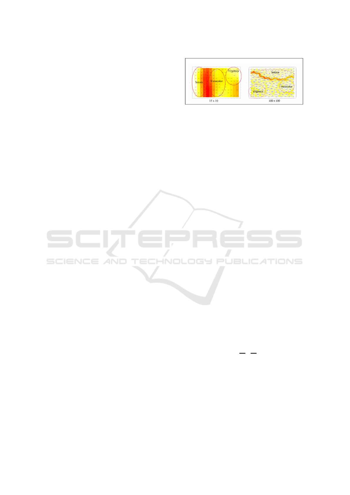
Our experiments demonstrate that our parallel al-

gorithm is better suited for highly computational de-

manding maps, such as the maps generated with large

SOMs. Using a large number of neurons provides

a higher resolution clustering of the data and facil-

itates the pattern recognition during the analysis, as

shown in Figure 1. Furthermore, the maps produced

by the Par-VSOM are equivalent in quality to the

maps produced by the original SOM iterative algo-

rithm. The current Par-VSOM model is parallel and

multi-threaded, and therefore well suited as a replace-

ment for other parallel algorithms to train the self-

organizing maps.

The paper is organized as follows: In Section

2, we start our discussion with an overview of the

SOM and a brief introduction to the VSOM (Hamel,

2019) vectorized rules, which can be viewed as an im-

plementation of a competitive learning scheme com-

prised of a competitive step and an update step with

vector and matrix training. The relevant details about

related research work are included in Section 3. As

part of Section 4, we develop the Par-VSOM vector-

based parallel training and examine the data level par-

allelisms achievable using vectorized single instruc-

tion with multiple data (SIMD) registers and discuss

the limitations. Under Section 5, we included the

study of the performance of our parallel vectorized

Rivera-Morales, O. and Hamel, L.

Par-VSOM: Parallel and Stochastic Self-organizing Map Training Algorithm.

DOI: 10.5220/0011377700003332

In Proceedings of the 14th International Joint Conference on Computational Intelligence (IJCCI 2022), pages 339-348

ISBN: 978-989-758-611-8; ISSN: 2184-3236

339

training implementation by comparing it to various

CPU and GPU SOMs variants. Finally, in Section 6,

we conclude our discussion with a summary of the ob-

servations and some future research ideas under con-

sideration.

2 THE SOM AND VSOM

ALGORITHMS

The origins of the self-organizing maps model can be

traced back to the Vector Quantization (VQ) method

(Kohonen, 2001). The VQ is a signal-approximation

algorithm that approximates a ﬁnite “codebook” of

vectors m

∈ R

, i = 1, 2, ..., k to the distribution of the

input data vector x ∈ R

. In the SOM context, the

approximated codebook allows us to categorize the

nodes and forms an “elastic network,” which becomes

a meaningful, coordinated map or grid system.

From a computational perspective, the SOM can

be described as a mapping of high dimensional in-

put data onto a low dimensional neural network pro-

jected as a 2D or three-dimensional (3D) constrained

topological map (Hastie et al., 2001). The map-

ping is accomplished by assuming that the input data

set is a real vector such as x

= [ξ

, ξ

, ..., ξ

]

∈

. The SOM neuronal map can be deﬁned as a

model containing the parametric real vector m

, u

, ..., u

]

∈ R

associated with the neurons’

weights. If we consider the distance between the in-

put vector x

and the neuron vector m

then we can es-

tablish an initial minimum distance relation between

the input and the neurons by calculating the Euclidean

distances. Then, these distances are used to identify

the best matching unit (BMU) index with equation

(1).

c = argmin

(||m

− x

) (1)

To deﬁne the SOM in terms of matrix and vector

operations it is assumed that the map’s neurons are

stored in a n×d matrix M where each row i represents

the neuron m

with d components,

M[i, ] = m

= (m

, . . . , m

)

, (2)

with i = 1, . . . , n. The training data x consists of a

set D= {x

, . . . , x

}. The set can be deﬁned as a l × d

matrix where each row k represents the training vector

with d components,

D[k, ] = x

= (x

, . . . , x

)

, (3)

with k = 1, . . . , l.

Essential details to consider include (1) the dimen-

sionality d for the input, and (2) the neuron vectors

Figure 1: IRIS 15x10 small SOM and IRIS 100x100 large

SOM, neuronal heatmaps patterns with different resolu-

tions.

are required to be the same size for well-deﬁned ma-

trix operations.

2.1 The SOM and VSOM Competitive

Step

In the competitive step, we ﬁnd the BMU for a partic-

ular training instance x

. In the classic SOM we use

an iterative process to ﬁnd the BMU using 1. Here

the i = 1, 2, ..., n represents the index of the neurons

in the map and m

represents the neuron in index i.

The argmin is a function that returns the minimum

value and c contains the index of the BMU.

In the VSOM context this step requires us to cal-

culate the Euclidean distance as a set of vector and

matrix operations. These operations ﬁnd the c in-

dex associated with the neuron with the minimum dis-

tance to the training instance. The BMU c index cor-

responds to the neuron in the map with the highest

resemblance to the particular x

selected for training

during the epoch.

The ﬁrst step to calculate the BMU requires us

to compute a matrix X to hold a randomly selected

training vector. The matrix X in equation (4) is de-

ﬁned with a component sizes of n × d, where each

row is holding the current epoch training vector x

, x

, . . . , x

)

, which is randomly selected from ma-

trix D,

X = 1

⊗ x

. (4)

Here, the symbol ⊗ represents the outer product and

is a column vector deﬁned as,

= (1, 1, . . . , 1

| {z }

)

. (5)

Since 1

is a column vector and x

is a row vector the

operation in (4) is well deﬁned. After populating the

instance matrix X with the duplicated x

values, equa-

tions (6), (7) and (8) are used to compute the square of

the Euclidean distances between all the map neurons

and the selected input vector,

∆ = M − X (6)

Π = ∆ ◦ ∆ (7)

s = Π × 1

(8)

NCTA 2022 - 14th International Conference on Neural Computation Theory and Applications

340

In equation (6) we calculate the difference between

the matrices with an element-by-element matrix sub-

traction. In equation (7) we use the Hadamard product

to allow us to calculate the Π matrix, in this context

◦ represents the element-by-element matrix product

and X, M, ∆ and Π are all n × d matrices.

Lastly, in equation (8) we use a ‘row sum’ matrix

reduction to compute the vector s of size n. Here, 1

a column vector similar to (5) with the dimensionality

deﬁned by the value of d.

2.2 The SOM and VSOM Update Step

In the classic stochastic SOM, after completing

the BMU calculations, the updates to the neuronal

weights are accomplished using the training instance

to inﬂuence the best matching neuron and its sur-

rounding neighborhood.

← m

− η(m

− x

)h(c, i) (9)

The weights update step in equation (9), affects

every neuron inside the neighborhood radius of inﬂu-

ence. Here, the learning rate η serves as a scaling

factor between 0 and 1. The h(c, i) acts as the loss

function , where i = 0, 1, ... , n and it can be deﬁned

as,

h(c, i) =



1 if i ∈ Γ(c),

0 otherwise,

(10)

where Γ(c) is the neighborhood of the best matching

neuron m

with c ∈ Γ(c). In the classic SOM, the

learning factor and the loss function both decreased

monotonically over time (Kohonen, 2001).

In the VSOM, the update step for all the neurons

in the map is accomplished with matrix operations

and is deﬁned as,

M ← M − η∆ ◦ Γ

. (11)

Here, η is the learning rate, ∆ contains the calcula-

tions of the difference between the neurons and the

selected training instance as computed in (6), and

the symbol ◦ represents the Hadamard product. The

Hadamard product represent by ◦ is the element-by-

element matrix product. Similarly to the SOM, in

the VSOM, the learning rate η is linearly reduced as

epochs increase.

However, our experimental results demonstrate

that a constant learning rate η generates higher quality

convergence indexes in large map instances. Initially,

the update rule for each best matching neuron has

a very large radius of inﬂuence and includes all the

neurons on the map. After multiple training epochs,

the neighborhood radius around the BMU gradually

Figure 2: SOM preserving the neighborhood topology in

3D space (Hastie et al., 2001).

shrinks to the point that the ﬁeld of inﬂuence only in-

cludes the best matching neuron m

as shown in (12).

Γ(c)|

t0

= {c}. (12)

The competitive and the update steps are com-

puted during each epoch using the randomly selected

training instances until some convergence criterion is

fulﬁlled. After reaching a maximum convergence, ev-

ery data point will be assigned to an speciﬁc data neu-

ron forming clusters in the grid and preserving the

neighborhood topology as shown in Figure 2.

Algorithm 1 and 2 summarizes the matrix and

vector operations required for the parallel Par-VSOM

training. For a more detailed explanation of the SOM

and VSOM algorithms, see reference (Hamel, 2019).

3 RELATED WORK

In this section, we look at prior work related to par-

allel SOM algorithms and its applications. Recent

parallel self-organizing maps research has demon-

strated promising improvements using various paral-

lel methods. Some of the methodology mentioned in

current scientiﬁc publications on this topic include:

combining data and network partitioning techniques

(Richardson and Winer, 2015; Silva and Marques,

2007), exploiting cache effects (Rauber and Merkl,

2000), using map-reduce programming paradigm

(Sarazin et al., 2014; Sul and Tovchigrechko, 2011;

Schabauer and Weishaupl, 2005), replacing the SOM

iterative construct with vector and matrix operations

(Hamel, 2019), and using various types of acceler-

ated architectures for parallelism (Davidson, 2015;

Moraes et al., 2012; Abadi et al., 2016; Mancini et al.,

2020; Wittek et al., 2013). In addition, recent publi-

cations demonstrate how to utilize SOM as a pattern

recognition tool (Kim et al., 2020; Li et al., 2018b;

Lokesh et al., 2019). In general, recent research pub-

lications share similars goals such as: ﬁnding new

applications, improving optimal performance and in-

creasing speed-up using different SOM approaches.

Par-VSOM: Parallel and Stochastic Self-organizing Map Training Algorithm

341

3.1 SOM Parallel Hybrid Methods

The combination of data and network partitioned par-

allel methods develop by Richarson et al. (Richard-

son and Winer, 2015) splits up the map to compute

the best matching calculation and nodes update on

separate threads. This hybrid methodology also di-

vides the data amongst individual threads for data par-

tition parallelism. As part of their research ﬁndings,

they concluded that parallelizing the classic SOM al-

gorithm using such techniques in a GPU can save

computation time and increase the speed-up by nearly

15X in maps with 10,000 points and 5 dimensions. A

similar method was proposed by (Silva and Marques,

2007), achieving a performance increases of 1.27X

training large maps on a small HPC cluster.

3.2 SOM Vectorization

The VSOM by (Hamel, 2019) replaced all the iter-

ative constructs of the standard stochastic SOM al-

gorithm with vector and matrices operations. The

VSOM implementation resulted in a performance in-

crease of up to 60X faster after running 10000 itera-

tions in a 25 X 20 map. Since the VSOM seems to be

offering the highest speed-up increase of all the cur-

rent SOM research publications, our research is focus

on the parallelization of the VSOM algorithm and its

implementation in hardware accelerators.

3.3 SOM in Multiple Parallel

Architectures

Among the SOM parallel approaches previously dis-

cussed, not many offer an available open source

repository to validate the research ﬁndings or con-

tinue with further investigations. In this paper, we

decided to compare our proposed parallel implemen-

tation with some of the widely available parallel SOM

projects packages. As part of the GPU comparisons

we utilize, Quicksom (Mallet et al., 2021a) which

offers a parallel GPU Batch-SOM algorithm imple-

mented using the Python PyTorch framework and

speed-ups results showed at least a 20 speed-up over

the CPU version using bioinformatics datasets (Mal-

let et al., 2021b). In addition, we also included a com-

parison with XpySom (Mancini et al., 2020) a paral-

lel Batch-SOM variant implemented using the Google

Tensorﬂow 2.0 framework and Python Numpy li-

brary. The XpySom package is based on the Mini-

som(Vettigli, 2021), a non-parallel, minimalistic and

Numpy based widely know implementation of the

SOM. The XpySom research paper (Mancini et al.,

2020) indicates their parallel variants outperforms the

popular SOM GPU package Somoclu by two and

three orders of magnitude.

4 Par-VSOM: PARALLEL

VECTORIZED SOM

4.1 Hardware for Parallel Vectorization

Our novel parallel implementation is based on the

VSOM algorithm proposed by (Hamel, 2019). On the

VSOM, the stochastic SOM training is redeﬁned to

execute as a set of vector and matrix operations. Since

all the matrix data elements are independent of each

other, they can be executed as coarse-grained “embar-

rasingly parallel” tasks to exploit multiple hardware

threads (or cores) available in the devices (Jaaske-

lainen, 2019). In the VSOM context, the vectoriza-

tion of the calculations can be implemented as vector

instructions, which are also known as SIMD instruc-

tions and are a form of Data-Level Parallelism. These

vector instructions apply the same operation over

multiple data elements (like integers and ﬂoating-

point values) concurrently, given that these items are

stored contiguously in vector/SIMD registers (Pilla,

2018). In modern Intel and AMD CPU architectures,

these vector instructions are known as Advance Vec-

tor Extensions (AVX), AVX2, AVX-512 instructions

set and Streaming SIMD Extensions (SSE4).

In contrast, the GPUs with their substantial

amount of nodes allows for the creation of thousands

of threads to perform vector calculations simultane-

ously. Furthermore, the current NVIDIA GPUs can

access there memory much faster when accessing ad-

jacent data concurrently. This is optimized when

groups of 32 GPU threads or warps do the request

simultaneously, causing “memory coalescing” (Dick-

son et al., 2011).

4.2 Par-VSOM Algorithm

In the classic SOM with iterative operations, the op-

erations per column are solved in a loop structure

sequentially. This serial approach results in high

overhead and additional latency during every training

epoch. Conversely, the VSOM vector and matrix op-

erations are vectorized by the compiler, and they are

executed in the CPU as vector operations. To illus-

trate, in a data set with 32 instances, the VSOM using

vectorized operations will need to execute a total of

four “minus” operations to compute a ∆ matrix en-

tirely. Using the VSOM vectorization, the ∆ matrix

“minus” operation can be completed with a speed-up

NCTA 2022 - 14th International Conference on Neural Computation Theory and Applications

342

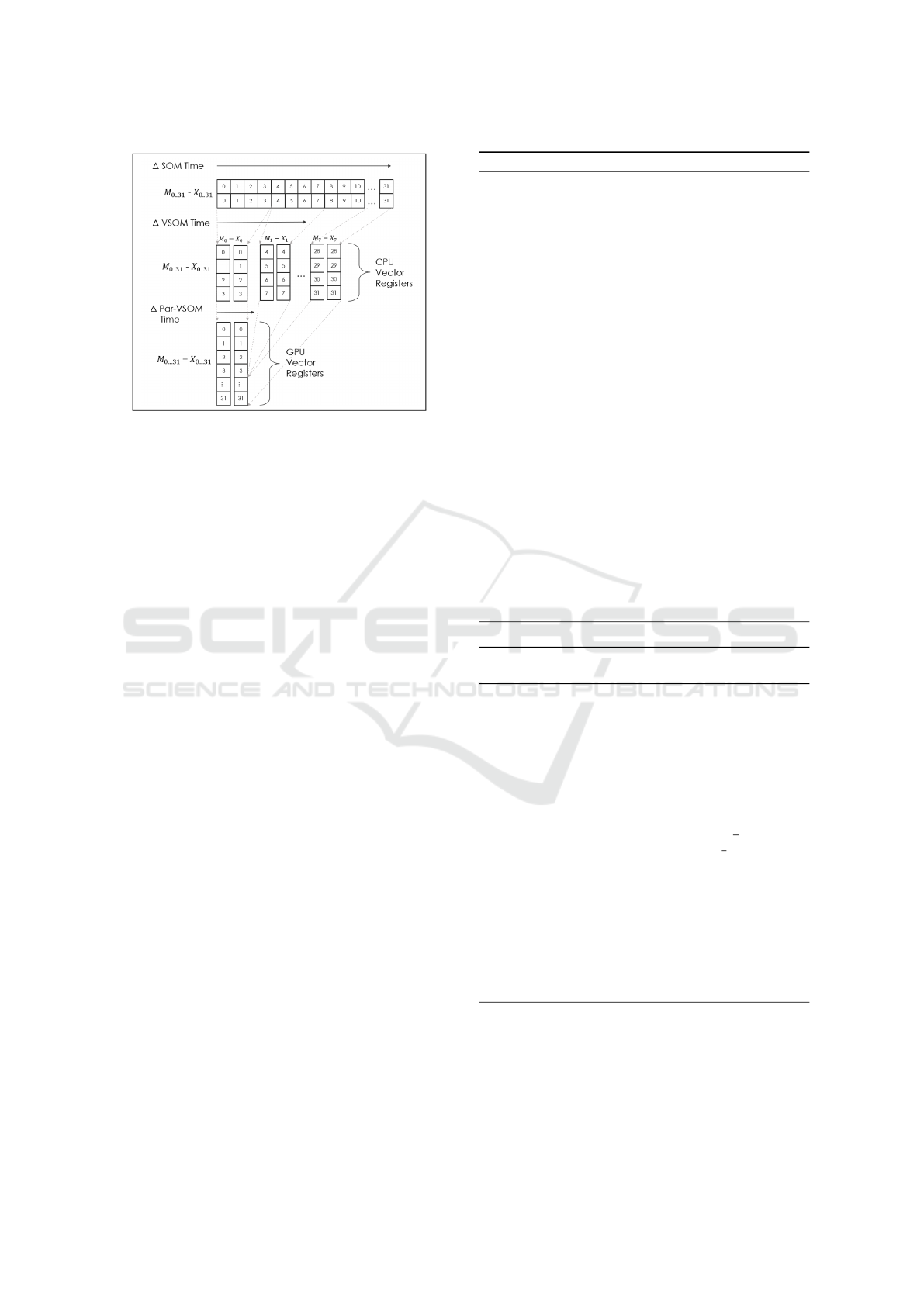
Figure 3: The time comparison of ∆ calculation during

the competitive step for SOM, VSOM, and PAR-VSOM

demonstrate modern architecture advances in vectorization

capability increases the primitive operations’ overall speed-

up performance.

increase of 4X compared to the SOM, as illustrated in

Figure 3.

In the Par-VSOM, the vector and matrix opera-

tions of the original VSOM are replaced with parallel

computational kernels executing in a hardware accel-

erator architecture. The parallel kernels manipulate

the matrices columns in a uniﬁed vector V

as shown

in equation (13). In the kernel, the matrices are ex-

pressed as tuples of column vectors and encapsulated

into one unifying vector. Based on the data of our ex-

ample in Figure 3, the unifying vector technique will

result in executing the 32 elements operation in one

single vectorized operation, providing a performance

increase of 128x.

[i ∗ n] = (t

, . . . ,t

)

∪ (t

, . . . ,t

)

. . . ∪ (t

, . . . ,t

)

(13)

In the unifying vector equation (13), we have

shown how the matrices can be express in terms of

union of tuples. Here, ∪ represents the union oper-

ator. In the Par-SOM algorithm (1) and (2), we are

assuming all the matrices of the VSOM are imple-

mented as a data structure consisting of multiple tu-

ples (t

, ...,t

) where each column is represented

by the tuple (t

)

with i representing the dimensional-

ity of the matrix and n the number of instances. This

technique allows the data-level parallelism to occur

by executing all the matrix operations as optimized

vector operations inside the Φ kernels as presented in

algorithm 1 and 2.

In our GPU implementation, we decided to use

CUDA Thrust. Considering that the Par-VSOM is a

parallel and vectorized implementation of the VSOM

algorithm, the Thrust template is an ideal candidate

Algorithm 1: The Par-VSOM training algorithm.

1: Given:

2: D ← {training instances, a l x d matrix}

3: M ← {neurons, a n x d vector of tuples}

4: η ← {learning rate 0 < η < 1}

5: Γ(c) ← {neighborhood function for some neuron c}

6: minIndex(s) ← {returns location of min. val in s}

7: Φ ← {Vectorized kernel operation, with all matrices

8: columns uniﬁed as tuples in a single column vector.}

9: Repeat

10: /***Select a matrix training instance as vector

11: for some k = 1, ..., l and f = 1, ..., d : ***/

12:

13: x

← D[k][1] ∪ D[k][2]... ∪ D[k][ f ]

14:

15: /***Find the winning neuron using kernels ***/

16: X ← Φ

⊗ x

)

17: ∆ ← Φ

∆

(M − X)

18: Π ← Φ

(∆ ◦ ∆)

19: /***Sum of vector subsections (rowsum) ***/

20: s ← Φ

(Π

1...(n∗1)

+ Π

(n∗1)...(n∗2)

21: ... Π

(n∗(d−1)...(n∗d)

)

22: c = minIndex(s)

23:

24: /***Update neighborhood with vector operations ***/

25: Γ

← Φ

(Γ(c))

26: M

new

← Φ

new

current

− η∆ ◦ Γ

)

27: Until done

28: return M

new

Algorithm 2: The Par-VSOM Neighborhood Function Γ(c)

as mentioned in equation (10) and (11).

1: Given:

2: c ← {index of winning neuron}

3: n ← {the number of neurons on the map}

4: nsize ← {neighborhood radius}

5: P ← {an n × 2 vector with p

= P[i, ] = (x

, y

)}

6: 1

← {constant column vector with value 1}

7: 0

← {constant column vector with value 0}

8: Φ ← Vectorized kernel operation, with all matrices

9: columns uniﬁed as tuples in a single column vector.

10: x ← { x values in ﬁrst section: 1,...,(

− 1)}

11: y ← { y values in second section:

, ..., (n × 2)}

12:

13: P

← Φ

(P[c, ])

14: C ← Φ

⊗ p

)

15: ∆ ← Φ

∆

(P − C)

16: Π ← Φ

(∆ ◦ ∆)

17: /***Perform rowsum with vector subsections

18: d ← Φ

(Π

+Π

)

19: hood ← Φ

hood

(ifelse(d < (nsize × 1.5)

, 1

, 0

))

20: return hood

due to the vast number of vector functions available.

In addition, Thrust manages all the CUDA kernel

initialization, memory transfers and allocation in the

background, and provides highly optimized libraries

for vector operations (Nvidia.com, 2020).

Par-VSOM: Parallel and Stochastic Self-organizing Map Training Algorithm

343

Since most of the VSOM algorithm consists of

matrix operations, we utilized Thrust specialized

transformation and reduction functions to process the

matrices as vectors. In the case of a matrix with three

columns, storing 3d points as an array of ﬂoat3 in

CUDA is generally a bad idea, since array accesses

are not properly coalesced (Nvidia.com, 2020). To

address this memory access issue, the number of rows

n was used as a delimiter to identify the beginning and

the end of each column in the unifying vector Vu. The

column-wise encapsulation of the matrix transforms

the three-dimensional columns in to one Vu vector.

This allows coalesced memory access and faster op-

eration execution.

One of the important differences between the orig-

inal VSOM algorithm and the Par-VSOM algorithm ,

is the data structure manipulation during the selection

of the D matrix random training instance algorithm 1

(line 13). Here, the training computation transforms

the selection into an X

vector that includes all the

matrix D columns and allows us to ﬁnd the BMU us-

ing vector operations. To be able to use the optimized

“minIndex(s)” function in line 22, we reduced the Π

vector with length n∗d into a vector of length n, using

operations equivalent to a rowsum across d dimen-

sions in line 20.

Similarly, the Par-VSOM neighborhood Function

Γ in algorithm 2, emulates the rowsum operations of

algorithm 1 in line 18 by utilizing the vector elements

representing the x and y columns accordingly and re-

turns one vector that includes the distances of the neu-

rons in the grid. In lines 19 to 20 using the computed

distances, the vector neighborhood determination is

performed and return a hood vector that activates the

neurons considered to be part of the neighborhood by

ﬂipping to “1” their corresponding neurons index.

4.3 Limitations

4.3.1 Large Computational Workloads

The Par-VSOM is recommended for clustering prob-

lems requiring high computational workloads. To ob-

tain our experimental results, we tested with multiple

datasets and various map sizes. The results demon-

strated the Par-VSOM is not suitable for small maps,

low-dimensional datasets, or minimal computational

workloads. Here, we assume the users will have a

GPU hardware accelerator available as part of their

setup.

In general, Big data and other extensive datasets

analysis requires generating large neuronal maps as

part of the pattern analysis and clusters visualizations.

The GPUs have become one of the default tools to

process high complexity problems and are easily ac-

cessible in cloud environments, but we are aware that

not everyone may have access to one.

5 EXPERIMENTS

5.1 Hardware Setup

All the Par-VSOM, Xpysom and Quicksom parallel

experiments were performed using the Amazon AWS

cloud service instances with Linux and Deep Learn-

ing Amazon Machine Images (AMI). The sequential

CPU experimental setting included an Intel I7-7700K

running at 4.20 GHz/ 4.50GHz turbo with four cores

and capable of executing eight threads. The GPU tests

were performed in an AWS P3.2xlarge with 18 virtual

Intel Xeon E5 2686 CPU operating at 2.7 GHz/ 3.0

GHz turbo and an NVIDIA Tesla V100. The Tesla

V100 contains 5120 NVIDIA Cuda cores with 16 Gb

of HBM2 memory. The Tesla V100 memory clock

setting was 877 Mhz with memory graphics clocked

at 1530 Mhz.

5.2 Par-VSOM Setup and

Hyper-parameters

The experimental setup utilized the default values

of the SOM and VSOM Popsom (Hamel et al.,

2016). For the Quicksom(Mallet et al., 2021b)

and Xpysom(Mancini et al., 2020) BatchSOM pack-

ages, we maintained the learning rate constant to ob-

tain higher convergence indexes and tune the hyper-

parameters as deﬁned in Table 1.

Table 1: Par-VSOM Hyper-Parameters.

**Hyper-Parameters** **Values**

Training Iterations 1 × 10

... 1 × 10

Learning Rate η 0.7

Neighborhood Radius Bubble, Gaussian(for Quicksom)

Map sizes 15x10, 150x100, 200x150

Datasets Iris, Epil, WDBC

As part of our tests, we compared the performance

and the quality of the maps generated by our parallel

Par-VSOM with two CPU SOM and two GPU SOM

variants. The quality of the maps is based on the con-

vergence index as deﬁne in (Tatoian, 2018). The CPU

single-node tests used the SOM and the VSOM al-

gorithms included as part of the R language Popsom

package with C bindings applications. In contrast, the

parallel comparisons were done using the two GPU-

based SOM packages; Quicksom with Python 3, Py-

torch 1.4 and Xpysom using Tensorﬂow 2.0 in their

NCTA 2022 - 14th International Conference on Neural Computation Theory and Applications

344

Table 2: Times and Speed-up gains of the Par-VSOM for different training algorithms using a 200 × 150 map.

iter Time Time Time Time Time Speed-up Speed-up Speed-up Speed-up

SOM(s) VSOM(s) P-VSOM(s) Xpysom(s) Quicksom(s) Par-VSOM/ Par-VSOM/ Par-VSOM/ Par-VSOM/

CPU CPU GPU CPU-GPU CPU-GPU SOM VSOM Xpysom Quicksom

R\C R\Fortran Cuda Thrust TensorFlow PyTorch

*** Iris D=4***

1 1.148 0.035 0.027 0.301 0.257 42.5 1.3 11.1 9.5

10 1.350 0.046 0.029 0.319 0.257 46.6 1.6 11.0 8.9

100 2.362 0.067 0.049 0.414 0.434 48.2 1.4 8.4 8.9

1000 13.447 0.324 0.235 1.408 2.32 57.2 1.4 6.0 9.9

10000 124.011 2.756 1.925 10.742 21.456 64.4 1.4 5.6 11.1

100000 1228.811 26.210 18.275 110.900 212.791 67.2 1.4 6.1 11.6

*** Epil D=8***

1 1.831 0.053 0.046 0.300 0.262 39.8 1.2 6.5 5.7

10 1.949 0.058 0.049 0.313 0.259 39.8 1.2 6.9 5.3

100 3.125 0.108 0.072 0.412 0.643 43.4 1.5 5.7 8.9

1000 14.854 0.554 0.294 1.411 4.667 50.5 1.9 4.8 15.8

10000 132.193 4.928 2.577 10.660 46.755 51.3 1.9 4.1 18.1

100000 1306.793 47.560 22.535 115.372 462.908 58.0 2.1 5.1 20.5

*** WDBC D=30***

1 0.966 0.152 0.125 0.303 0.262 7.7 1.2 2.4 2.0

10 1.167 0.165 0.130 0.319 0.256 9.0 1.3 2.5 2.0

100 3.161 0.342 0.174 0.416 0.762 18.2 2.0 2.5 4.4

1000 23.236 2.076 0.601 1.387 6.386 38.7 3.5 2.3 10.6

10000 222.034 19.105 4.712 11.389 63.871 47.1 4.1 2.4 13.6

100000 2224.134 188.080 46.114 111.223 634.687 48.2 4.1 2.4 13.8

Table 3: Quality of maps produced by the different training algorithms (SOM=Classic SOM, VSM=VSOM, P-V=Par-VSOM,

X-P=Xpysom, Q-S=Quicksom and D=Dimensions).

iter 15x10 150x100 200x150

SOM VSM P-V X-P Q-S SOM VSM P-V X-P Q-S SOM VSM P-V X-P Q-S

*** Iris, D=4***

1 |0.50 0.15 0.09 0.50 0.45| |0.41 0.00 0.00 0.50 0.12| |0.40 0.00 0.00 0.50 0.08|

2 |0.43 0.53 0.48 0.37 0.49| |0.02 0.45 0.49 0.50 0.50| |0.34 0.45 0.49 0.47 0.50|

3 |0.92 0.95 0.93 0.88 0.48| |0.42 0.79 0.49 0.40 0.50| |0.12 0.85 0.77 0.32 0.50|

4 |0.93 0.91 0.91 0.92 0.37| |0.92 0.91 0.96 0.28 0.48| |0.92 0.93 0.91 0.29 0.48|

5 |0.95 0.94 0.94 0.87 0.27| |0.96 0.99 0.95 0.26 0.41| |0.90 0.99 0.97 0.32 0.37|

*** Epil, D=8***

1 |0.03 0.14 0.15 0.72 0.40| |0.12 0.00 0.00 0.46 0.06| |0.12 0.00 0.0 0.46 0.13|

2 |0.70 0.56 0.40 0.60 0.48| |0.03 0.45 0.45 0.49 0.50| |0.07 0.38 0.40 0.50 0.50|

3 |0.92 0.92 0.94 0.81 0.80| |0.31 0.68 0.53 0.36 0.50| |0.27 0.40 0.64 0.41 0.50|

4 |0.94 0.92 0.93 0.65 0.79| |0.45 0.48 0.68 0.29 0.86| |0.85 0.60 0.56 0.40 0.56|

5 |0.96 0.91 0.93 0.95 0.78| |0.85 0.97 0.96 0.40 0.84| |0.91 0.98 0.93 0.38 0.54|

*** WDBC, D=30***

1 |0.31 0.14 0.11 0.68 0.37| |0.00 0.00 0.00 0.62 0.13| |0.07 0.00 0.00 0.50 0.00|

2 |0.50 0.53 0.50 0.67 0.66| |0.08 0.51 0.45 0.53 0.55| |0.27 0.55 0.44 0.50 0.50|

3 |0.90 0.92 0.88 0.50 0.80| |0.30 0.48 0.64 0.40 0.66| |0.40 0.60 0.63 0.40 0.50|

4 |0.92 0.90 0.90 0.69 0.67| |0.47 0.81 0.80 0.43 0.89| |0.52 0.85 0.85 0.44 0.50|

5 |0.89 0.92 0.93 0.68 0.68| |0.88 0.90 0.91 0.37 0.76| |0.81 0.97 0.98 0.37 0.50|

implementation.

For our experiments we used three real-world

datasets to train our algorithms:

1. Iris (Fisher, 1936) - a dataset with 150 instances

and 4 attributes that describes three different

species of Iris.

2. Epil (Thall and Vail, 1990) - a dataset on two-

week seizure counts for 59 epileptics. The data

consists of 236 observations with 8 attributes. The

dataset has two classes - placebo and progabide, a

drug for epilepsy treatment.

3. Wisconsin Breast Cancer Dataset (wdbc) (Street

et al., 1993) - a dataset with 30 features and 569

instances related to breast cancer in Wisconsin,

for our experiment we generated a random nor-

malized sample of 100 instances. The dataset has

two classes: malignant and benign.

These datasets are purposely selected to test the

algorithm performance by increasing the dimension-

ality complexity of the input data. To measure the Par-

VSOM performance, we ran each timing test three

times and took the average time over these runs. The

times reported are the time required for the CPU to

perform the calculations and it is given in CPU sec-

onds. Similarly, the quality tests were done by aver-

aging three quality measurements using the conver-

gence index (CI) explain in detail in (Tatoian, 2018)

and included as part of the R Popsom Package (Hamel

et al., 2016). The CI provides a 0 to 1 numbering scale

to measure the maps’ quality, with 0 represents the

Par-VSOM: Parallel and Stochastic Self-organizing Map Training Algorithm

345

lowest quality and 1 the highest quality. Furthermore,

three map sizes were considered for these experi-

ments, 15×10 (small), 150×100 (medium), 200×150

(large), to see how the different implementations per-

form on different map sizes. In addition, we trained

with various number of training iterations (in pow-

ers of 10) to discover what type of effect a change of

training duration had on the implementations.

5.3 Results

In the large map environment results included in Ta-

ble 2, we see the recurrent speed-up gains of the al-

gorithm with larger maps. The large size of data

buffers require for the calculations, the CPU cache

memory size limitations and DDR4 lower clock rate

does present an performance impact for the SOM

and VSOM CPU variants. The large workload and

substantial computational resources available in the

GPU, allows the Par-VSOM performance scale fur-

ther. Here, the Par-VSOM achieves a speed-up of 67

in comparison to the SOM. The table results demon-

strates, the Par-VSOM achieves superior speed-up

in all the three datasets comparisons, surpassing the

speed rates of all the other algorithm implementa-

tions. In this large map environment, the Par-VSOM

surpassed the SOM with a 67, the VSOM with a 4.1,

Xpysom with 6.1 and the Quicksom by 20 speed-up

increase.

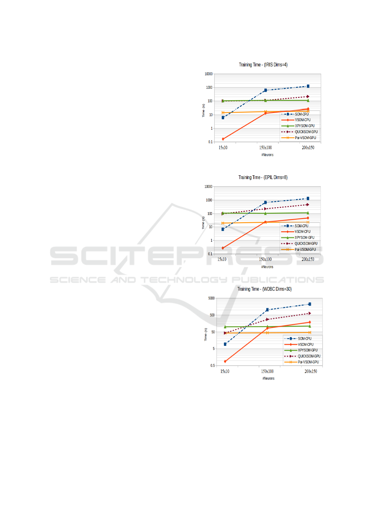
The training time charts included in Figure 4, cap-

ture a generalize representation of the overall results.

The Par-VSOM offers speedup performance increases

for the three datasets in medium and larger size maps

instances. The obtained results allows us to estab-

lish a direct relation between large neuronal maps and

better achievable times using the Par-VSOM. That is,

with a higher number of neurons an scalable speed up

can be achieved.

The Table 3 illustrates the baseline quality of orig-

inal algorithms using our three datasets. The results

present us with a recurring behaviour in most of the

maps, their is a pattern to decrease the convergence

quality when the datasets dimensionality increases.

However, we also identiﬁed as the size of the maps in-

creases, there is tendency for the vectorized variants

(VSOM and Par-VSOM) to generate higher quality

maps. Furthermore, our testing demonstrates Xpysom

and Quicksom SOM parallel versions can not reach

a high convergence index when larger map sizes are

used.

In terms of the quality of the maps, Figure 5 cap-

tures all the algorithm convergence indexes for the

three datasets. As illustrated, the Par-VSOM main-

tains relatively the same quality as the original SOM

(a) Iris Total Training Time at Convergence

(b) Epil Total Training Time at Convergence

Figure 4: Total training time for all datasets with multiple

map sizes at the convergence iteration 100000.

and the VSOM variants in all the maps. In contrast,

the parallel GPU BatchSOM variants (Xpysom and

Quicksom) only obtained good quality indexes with

smaller maps (15 x 10). In both of these parallel pack-

ages, the convergence index quality starts decreas-

NCTA 2022 - 14th International Conference on Neural Computation Theory and Applications

346

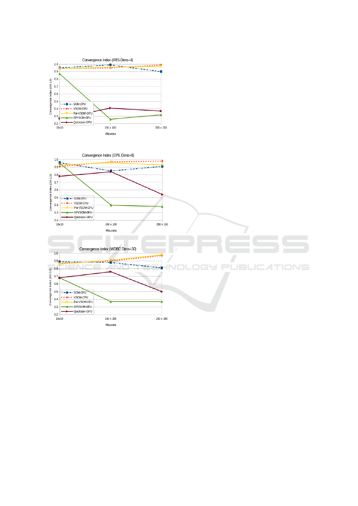
(a) Iris Convergence Index (Map Quality)

(b) Epil Convergence Index (Map Quality)

Figure 5: Convergence Index for the three datasets with var-

ious map sizes.

ing drastically after trying to organized medium and

larger SOM maps.

6 CONCLUSIONS

This work introduced the Par-VSOM, a highly par-

allel, vectorized and matrix-based implementation of

stochastic training for self-organizing maps. The

novel implementation presented here provides sub-

stantial performance increases over Kohonen’s itera-

tive SOM algorithm (up to 67 times faster), the CPU

based vectorized VSOM (up to 4 times faster), the

GPU Xpysom (up to 6.1 times) and Quicksom’s GPU

(up to 20 times) in large maps environments. The re-

sults clearly indicate the parallel BatchSOM approach

provided by Xpysom and Quicksom’s are no longer the

most optimal parallel option in newer architectures

due to the overhead and latency added by search for

winner in the batch algorithm. The performance gains

follow a direct relation with the increment of the map

sizes, as shown in Figure 4. Furthermore, the results

obtained by increasing the dimensionality and maps

sizes demonstrated the Par-VSOM provides a scal-

able speed-up performance when the neuronal map

size increases. In terms of the quality of the maps,

the maps produced by Par-VSOM approximates the

high quality values generated by the VSOM iterative

algorithms and original Kohonen’s SOM algorithm.

In the proposed design, the Par-VSOM is a multi-

threaded algorithm running in a GPU and therefore is

an adequate replacement for iterative stochastic train-

ing of SOM and parallel SOM variants. We are cur-

rently investigating how the Par-VSOM can be im-

plemented in an FPGA and what kind of performance

increase we can expect from this type of hardware ar-

chitecture. Based on our results, the Par-VSOM can

be viewed as an alternative to parallel SOM and a new

alternative for other parallel algorithms for clustering

and pattern recognition. In summary, since the train-

ing algorithms results demonstrate the produce maps

are roughly the same quality, the Par-VSOM provides

a parallel and high-performance alternative to SOM

algorithms. The Par-VSOM source code is available

at (Rivera-Morales, 2022).

REFERENCES

Abadi, M., Jovanovic, S., Ben Khalifa, K., Weber, S., and

Bedoui, M. (2016). A scalable ﬂexible som noc-based

hardware architecture. Advances in Self-Organizing

Maps and Learning Vector Quantization, pages 164–

175.

Barney, B. (2018). Introduction to Parallel Computing.

Lawrence Livermore National Laboratory.

Davidson, G. (2015). A parallel implementation of the self

organising map using opencl. University of Glasgow.

Dickson, N. G., Karimi, K., and Hamze, F. (2011). Impor-

tance of explicit vectorization for cpu and gpu soft-

ware performance. Journal of Computational Physics,

230(13):5383–5398.

Fisher, R. A. (1936). The use of multiple measurements in

taxonomic problems. Annals of eugenics, 7(2):179–

188.

Par-VSOM: Parallel and Stochastic Self-organizing Map Training Algorithm

347

Hamel, L. (2019). Vsom efﬁcient, stochastic self-

organizing map training. In Proceedings of the 2018

Intelligent Systems Conference (IntelliSys) Volume 2,

pages 805–821.

Hamel, L., Ott, B., and Breard, G. (2016). pop-

som: Functions for Constructing and Evaluating Self-

Organizing Maps. R package version 4.1.0.

Hastie, T., Tibshirani, R., and Friedman, J. (2001). The

Elements of Statistical Learning. Springer Series in

Statistics. Springer New York Inc., New York, NY,

USA.

Jaaskelainen, P. (2019). Task parallelism with opencl: A

case study. Journal of Signal Processing Systems,

pages 33–46.

Kim, K.-H., Yun, S.-T., Yu, S., Choi, B.-Y., Kim, M.-J.,

and Lee, K.-J. (2020). Geochemical pattern recogni-

tions of deep thermal groundwater in south korea us-

ing self-organizing map: Identiﬁed pathways of geo-

chemical reaction and mixing. Journal of Hydrology,

589:125202.

Kohonen, T. (2001). Self-organizing maps. Springer Berlin.

Li, J., Chen, B. M., and Lee, G. H. (2018a). So-net: Self-

organizing network for point cloud analysis. In Pro-

ceedings of the IEEE conference on computer vision

and pattern recognition, pages 9397–9406.

Li, T., Sun, G., Yang, C., Liang, K., Ma, S., and Huang, L.

(2018b). Using self-organizing map for coastal water

quality classiﬁcation: Towards a better understanding

of patterns and processes. Science of The Total Envi-

ronment, 628-629:1446–1459.

Lokesh, S., Kumar, P. M., Devi, M. R., Parthasarathy, P.,

and Gokulnath, C. (2019). An automatic tamil speech

recognition system by using bidirectional recurrent

neural network with self-organizing map. Neural

Computing and Applications, 31(5):1521–1531.

Mallet, V., Nilges, M., and Bouvier, G. (2021a). Quicksom.

https://github.com/bougui505/quicksom.

Mallet, V., Nilges, M., and Bouvier, G. (2021b). quick-

som: Self-organizing maps on gpus for clustering

of molecular dynamics trajectories. Bioinformatics,

37(14):2064–2065.

Mancini, R., Ritacco, A., Lanciano, G., and Cucinotta, T.

(2020). Xpysom: high-performance self-organizing

maps. In 2020 IEEE 32nd International Symposium

on Computer Architecture and High Performance

Computing (SBAC-PAD), pages 209–216. IEEE.

Moraes, F. C., Botelho, S. C., Duarte Filho, N., and Gaya,

J. F. O. (2012). Parallel high dimensional self orga-

nizing maps using cuda. In 2012 Brazilian Robotics

Symposium and Latin American Robotics Symposium,

pages 302–306. IEEE.

Mor

an, A., Rossell

o, J. L., Roca, M., and Canals, V. (2020).

Soc kohonen maps based on stochastic computing. In

2020 International Joint Conference on Neural Net-

works (IJCNN), pages 1–7.

Nvidia.com (2020). Thrust quick start guide. https://

docs.nvidia.com/cuda/thrust/index.html#abstract. Ac-

cessed: 2020-04-30.

Pilla, L. L. (2018). Basics of vectorization for fortran appli-

cations. Research Report, RR-9147:1–9.

Ramos, M. A. C., Leme, B. C. C., de Almeida, L. F.,

Bizarria, F. C. P., and Bizarria, J. W. P. (2017). Clus-

tering wear particle using computer vision and self-

organizing maps. In 2017 17th International Confer-

ence on Control, Automation and Systems (ICCAS),

pages 4–8.

Rauber, Andreas, P. T. and Merkl, D. (2000). parsom: a

parallel implementation of the self-organizing map ex-

ploiting cache efects: making the som ﬁt for interac-

tive high-performance data analysis. In Proceedings

of the IEEE-INNS-ENNS International Joint Confer-

ence on Neural Networks. IJCNN 2000, volume 6.

Richardson, T. and Winer, E. (2015). Extending paralleliza-

tion of the self-organizing map by combining data and

network partitioned methods. Advances in Engineer-

ing Software, 88:1–7.

Rivera-Morales, O. (2022). Par-vsom. https://github.com/

oxrm/Par-vsom.

Sarazin, T., Azzag, H., and Lebbah, M. (2014). Som clus-

tering using spark-mapreduce. In 2014 IEEE Interna-

tional Parallel & Distributed Processing Symposium

Workshops, pages 1727–1734. IEEE.

Schabauer, Hannes, E. S. and Weishaupl, T. (2005). Solv-

ing very large traveling salesman problems by som

parallelization on cluster architectures. In Sixth In-

ternatioanl Conference on Parallel and Distributed

Computer Applications and Technologies PDCAT’ 05,

pages 954–958. IEEE.

Silva, B. and Marques, N. (2007). A hybrid parallel som

algorithm for large maps in data-mining. New Trends

in Artiﬁcial Intelligence.

Street, W. N., Wolberg, W. H., and Mangasarian, O. L.

(1993). Nuclear feature extraction for breast tumor

diagnosis. In IS&T/SPIE’s Symposium on Electronic

Imaging: Science and Technology, pages 861–870. In-

ternational Society for Optics and Photonics.

Sul, S.-J. and Tovchigrechko, A. (2011). Parallelizing blast

and som algorithms with mapreduce-mpi library. In

2011 IEEE International Symposium on Parallel and

Distributed Processing Workshops and Phd Forum,

pages 481–489. IEEE.

Tatoian, R.and Hamel, L. (2018). Self-organizing map con-

vergence. International Journal of Service Science,

Management, Engineering, and Technology (IJSS-

MET), 9(2):61–84.

Thall, P. F. and Vail, S. C. (1990). Some covariance models

for longitudinal count data with overdispersion. Bio-

metrics, pages 657–671.

Vettigli, G. (2021). Minisom. https://github.com/

JustGlowing/minisom.

Wittek, P., Gao, S. C., Lim, I. S., and Zhao, L. (2013). So-

moclu: An efﬁcient parallel library for self-organizing

maps. arXiv preprint arXiv:1305.1422.

NCTA 2022 - 14th International Conference on Neural Computation Theory and Applications

348