A Comparative Study of Graph Neural Network Speed Prediction during

Periods of Congestion

Marko C. Oosthuizen

1,2 a

, Alwyn J. Hoffman

1 b

and Marelie H. Davel

1,2,3 c

Faculty of Engineering, North-West University, South Africa

Centre for Artiﬁcial Intelligence Research (CAIR), South Africa

National Institute for Theoretical and Computational Sciences (NITheCS), South Africa

Keywords:

Trafﬁc Prediction, Congestion, Graph Neural Network.

Abstract:

Trafﬁc speed prediction using deep learning has been the topic of many studies. In this paper, we analyse

the performance of Graph Neural Network-based techniques during periods of trafﬁc congestion. We ﬁrst

compare a selection of recently proposed techniques that claim to achieve good results using the METR-LA

and PeMS-BAY data sets. We then investigate the performance of three of these approaches – Graph WaveNet,

Spacetime Neural Network (STNN) and Spatio-Temporal Attention Wavenet (STAWnet) – during congested

periods, using recurrent congestion patterns to set a threshold for general congestion through the entire trafﬁc

network. Our results show that performance deteriorates signiﬁcantly during congested time periods, which

is concerning, as trafﬁc speed prediction is usually of most value during times of congestion. We also found

that, while the above approaches perform almost equally in the absence of congestion, there are much bigger

differences in performance during periods of congestion.

1 INTRODUCTION

Trafﬁc speed prediction forms an important element

of the management of metropolitan trafﬁc networks-

Deep neural networks are one of the most success-

ful techniques used for this purpose, and many differ-

ent approaches have been published in recent litera-

ture (Mena-Oreja and Gozalvez, 2020). The results of

trafﬁc speed prediction are used to advise both trafﬁc

authorities and road users about the best course of ac-

tion to limit or avoid congestion. As a result, predic-

tion accuracy is of most importance during times of

congestion, as little action is required from either road

users or the trafﬁc management system when trafﬁc is

ﬂowing normally.

When evaluating speed prediction methods dur-

ing both congested and not congested periods, it is

observed that prediction accuracy tends to deterio-

rate under congestion (Polson and Sokolov, 2017).

The high prediction accuracies claimed by many re-

searchers may therefore be somewhat misleading, as

the published performance levels are achieved when

https://orcid.org/0000-0003-2514-8135

https://orcid.org/0000-0003-4909-1073

https://orcid.org/0000-0003-3103-5858

averaging the performance of the model for congested

and not congested times, while much worse perfor-

mance is observed during periods when the prediction

algorithms are mostly needed.

In this paper, we evaluate state-of-the-art (SOTA)

deep learning trafﬁc speed prediction methods based

on their performance during periods of congestion.

The rest of the paper is organised as follows: Sec-

tion 2 contains a survey of related work. In Section

3 we describe the methodology and data used for the

study. Section 4 contains the results of the conges-

tion analysis, and in Section 5 we conclude and make

recommendations for future work.

2 BACKGROUND

Trafﬁc speed prediction attracts much attention be-

cause of the high costs associated with congestion in

big cities (Polson and Sokolov, 2017; Mena-Oreja and

Gozalvez, 2020). Due to lack of space and funds, it is

in most cases not possible to signiﬁcantly expand ex-

isting road networks in densely populated urban areas

(Shi et al., 2019). Other methods to address trafﬁc

congestion must therefore be considered.

Oosthuizen, M., Hoffman, A. and Davel, M.

A Comparative Study of Graph Neural Network Speed Prediction during Periods of Congestion.

DOI: 10.5220/0011374100003332

In Proceedings of the 14th International Joint Conference on Computational Intelligence (IJCCI 2022), pages 331-338

ISBN: 978-989-758-611-8; ISSN: 2184-3236

331

Trafﬁc congestion can be alleviated through more

effective trafﬁc management, as well as by providing

road users with more intelligent advice regarding the

routes to select to move from a speciﬁc origin to a spe-

ciﬁc destination (Nagy and Simon, 2018). One of the

primary information elements that enables more accu-

rate decision-making in such circumstances is knowl-

edge about future expected trafﬁc speeds on the dif-

ferent road sections forming part of the urban road

network (Xu et al., 2018). Such information can for

instance be used to modify the current cycle lengths

of trafﬁc lights (Gunawan and Chandra, 2014), or in-

crease the accuracy with which the expected travel

time along a speciﬁc route can be estimated (Gandhi

et al., 2020).

Deep neural networks have been proven to

outperform older techniques such as Autoregres-

sive Integrated Moving Average (ARIMA), vector

ARIMA, Support Vector Machines (SVMs) and oth-

ers (

Zliobait

e and Khokhlov, 2016). Different neural

network architectures have been developed for this

purpose, based on a variety of approaches includ-

ing Long-Short Term Memory (LSTM), adversarial

networks and graph-based networks (

Zliobait

e and

Khokhlov, 2016). A common requirement for these

techniques is the ability to simultaneously model both

temporal and spatial aspects of a network’s behav-

ior (Akhtar and Moridpour, 2021). Graph Neural Net-

work (GNN)-based techniques are particularly suc-

cessful, as discussed in more detail in Section 3.2.

Various authors have focused on trafﬁc speed pre-

diction during times of congestion (Zhou et al., 2020;

Chikaraishi et al., 2020). Mohanty (Mohanty, 2018)

found that trafﬁc congestion should be analysed as a

network-wide phenomenon. Large-scale spatial cor-

relation and long-term temporal correlation that gov-

ern trafﬁc congestion propagation across the regional

trafﬁc network may be exploited to develop conges-

tion prediction algorithms that are more effective than

local predictions. A method for the selection of alter-

native routes under trafﬁc congestion was proposed

by Xu et al. (Xu et al., 2018). They developed a deep

learning classiﬁer based on stacked Restricted Boltz-

man Machine layers followed by a backpropagation

layer. A method to predict decongestion time at rail

crossings was proposed by Jiang et al. (Jiang et al.,

2021). They used computer vision techniques to esti-

mate relevant features (such as the number of vehicles

waiting) in to measure and then model decongestion.

None of these works however speciﬁcally com-

pared different prediction approaches during periods

of congestion. This is recognised as a gap in existing

knowledge about trafﬁc prediction methods, which

we partially address here. Literature differentiates be-

tween two types of congestion: recurrent and non-

recurrent (Polson and Sokolov, 2017). In this pa-

per, we compare model performance during periods

of both recurrent and non-recurrent congestion.

3 METHODOLOGY

The analysis is conducted using the Los Angeles

Metropolitan Transportation Authority (METR-LA)

and Performance Measurement System (PeMS)-Bay

data sets, described in Section 3.1. We review SOTA

trafﬁc prediction systems (Section 3.2), and use this

to select an approach and establish a benchmark for

the study (Section 3.3). For the selected systems, we

perform a congestion analysis: demonstrating how

model performance differs during congested and not

congested periods, as well as how this changes as the

deﬁnition of network congestion changes.

3.1 Data Set and Task

The PeMS-Bay dataset consists of six months of

trafﬁc speed data aggregated into 5-minute win-

dows recorded using 326 sensors in the Bay area

of Los Angeles by California Transportation Agen-

cies (CalTrans) Performance Measurement System

(PeMS). The METR-LA dataset consists of four

months of trafﬁc speed data aggregated into 5-minute

windows recorded using 207 sensors on the highways

of Los Angeles. Both the PeMS-Bay and METR-LA

datasets are used to train trafﬁc forecasting models for

trafﬁc speed prediction. Both of the datasets, as sum-

marised in Table 1, were released by Li et al. (Li et al.,

2018) and are popular when evaluating trafﬁc predic-

tion models (Yang et al., 2021).

Table 1: Dataset characteristics.

METR-LA PeMS-Bay

Sensors 207 326

Period 4 months 6 months

Resolution 5 minutes 5 minutes

Speed unit miles per hour miles per hour

Time-steps 34 272 52 116

Along with the sensor readings, an adjacency ma-

trix, constructed from the pairwise road network dis-

tances between sensors adjusted using a thresholded

Gaussian kernel (Li et al., 2018), is also available for

each dataset.

NCTA 2022 - 14th International Conference on Neural Computation Theory and Applications

332

3.2 System Selection

To select a trafﬁc prediction system, we ﬁrst review

the published performance of prominent systems for

which implementations are publicly available. The

methods selected for evaluation are brieﬂy described

below.

The Spatial-Temporal Transformer Network

(STTN) consists of stacked spatial-temporal blocks

and a prediction layer (Xu et al., 2020). Each spatial-

temporal block consists of a spatial transformer and a

temporal transformer. In each spatial-temporal block,

the spatial transformer extracts spatial features from

the input node as well as the graph adjacency matrix.

The spatial transformer consists of a spatial-temporal

position embedding layer, a ﬁxed graph convolution

layer, a dynamic graph convolution layer and a gate

mechanism for information fusion.

Graph WaveNet implements a GNN for spatial-

temporal graph modelling by implementing an adap-

tive dependency matrix that does not require any prior

knowledge of the road network. By using stochas-

tic gradient descent the model discovers hidden spa-

tial dependencies by itself (Wu et al., 2019). Dilated

causal convolution is used in the temporal convolution

layer to capture temporal trends of nodes (Wu et al.,

2019).

STAWnet implements multiple stacked spatial-

temporal blocks and output layers. A spatial-temporal

block consists of a gated temporal convolution net-

work and a dynamic attention network. Dilated

causal convolution with a gate mechanism is used

for extracting temporal dependencies as for Graph

WaveNet. To dynamically model spatial dependen-

cies, the self-attention network is used on graph-

structured data to extract patterns in the model (Tian

and Chan, 2021).

Graph Multi-Attention Network (GMAN) fol-

lows the encoder-decoder architecture with a trans-

form attention layer added between the encoder and

decoder to convert the encoded historical trafﬁc fea-

tures to generate future representations. The encoder

and decoder are composed of spatial-temporal atten-

tion blocks (ST-attention blocks). The ST-attention

blocks are composed of a spatial attention mecha-

nism to model dynamic spatial correlations, a tem-

poral attention mechanism to model non-linear tem-

poral correlations, and a gated fusion mechanism

to adaptively fuse spatial and temporal representa-

tions (Zheng et al., 2020).

STNN implements spacetime interval learning to

explicitly capture intrinsic and latent spatio-temporal

correlations through a uniﬁed analysis of both spatial

and temporal features. To learn the spatial-temporal

correlations STNN combines novel spacetime atten-

tion blocks and spacetime convolution blocks (Yang

et al., 2021). The spacetime attention block high-

lights the interval between events capturing pair-wise

inﬂuences, and the spacetime convolution block ag-

gregates the learned features from spatial, temporal,

and spatial-temporal aspects to capture many-to-one

inﬂuences (Yang et al., 2021).

The published performance of these systems is

compared in Tables 2 and 3 for the METR-LA and

PeMS-Bay data sets, respectively. Performance is ob-

tained from the referenced papers as indicated in each

table.

3.3 Establishing a Benchmark

The ofﬁcial source code is available for STNN

GMAN

, STAWnet

, and Graph WaveNet

. An im-

plementation is available for STTN

as well but this

is not referenced by the original proposers of STTN.

Using the available software and settings as speciﬁed

by the authors, each of these systems was retrained

on the PeMS-Bay and METR-LA data sets, and the

recreated models evaluated on the ofﬁcial evaluation

sets. It was possible to recreate the results for Graph

WaveNet, STAWnet, and STNN. It was not possi-

ble to recreate the published results for either STTN

or GMAN without altering the available code. For

GMAN we experienced similar issues as were ob-

served by other forum users on Github, while the

STTN code was not being developed further at the

time of writing.

Only Graph WaveNet, STAWnet and STNN were

considered further. For these three models, the perfor-

mance of the published and recreated results is com-

pared in Tables 2 and 3 for the METR-LA and PeMS-

Bay tasks, respectively. Mean Absolute Error (MAE),

Root Mean Square Error (RMSE) and Mean Absolute

Percentage Error (MAPE) are reported, as deﬁned in

Eq. 1 to 3: x

is the predicted speed, y

is the true

speed over n measurements.

MAE =

∑

i=1

− x

(1)

RMSE =

∑

i=1

− x

)

(2)

MAPE =

∑

i=1

−x

(3)

https://github.com/libingixn/STNN

https://github.com/zhengchuanpan/GMAN

https://github.com/CYBruce/STAWnet

https://github.com/nnzhan/Graph-WaveNet

https://github.com/wubin5/STTN

A Comparative Study of Graph Neural Network Speed Prediction during Periods of Congestion

333

A negative percentage indicates that the published

results are better than the recreated results and vice

versa. Comparable results were achieved, verifying

the correctness of the implementations. However, it

was observed that the published results for STNN

were obtained using a different validation and test par-

tition than for the other techniques. In addition, per-

formance was determined by averaging over all the

prediction horizons up to the one reported on, whereas

the prediction errors for the other techniques are de-

termined at an individual prediction horizon only (a

single prediction, a speciﬁc number of steps into the

future). The STNN model was thus re-evaluated us-

ing the same test partition as Graph WaveNet and

STAWnet and the same performance measure as for

the other systems. (Note that neither the training data

nor the matching hyperparameters were changed but

that the correct validation set was used to select the

best-performing model from the training sequence.)

The change in the model itself had minimal effect, but

the change in evaluation measure had a signiﬁcant ef-

fect. This resulted in a decrease in performance, as

indicated by the STNN adjusted results in Tables 2

and 3. Graph WaveNet was therefore found to be the

best performing model with STAWnet producing very

similar results and STNN performing the worst of the

three.

4 ANALYSIS AND RESULTS

In this section, we analyse the performance of the

three methods for which the published results could

be recreated during periods of congestion.

4.1 Binned Trafﬁc Speed Analysis

To evaluate the performance of the different mod-

els during different congestion scenarios, we calcu-

late the MAE of the models’ predictions on different

ranges of trafﬁc speeds. We analyse this in two ways,

by considering the individual sensor speed and over-

all network speed as two different ways in which to

bin predictions. In the ﬁrst case, binned sensor speed

analysis, the MAE for all individual sensor predic-

tions that fall within a bin for a given horizon are

averaged. In the second case, binned average net-

work speed analysis, if the average network speed

falls within the bin, the MAE of all sensor predictions

at that time step are averaged, irrespective of individ-

ual sensor speeds. In both cases, each prediction hori-

zon is kept separate.

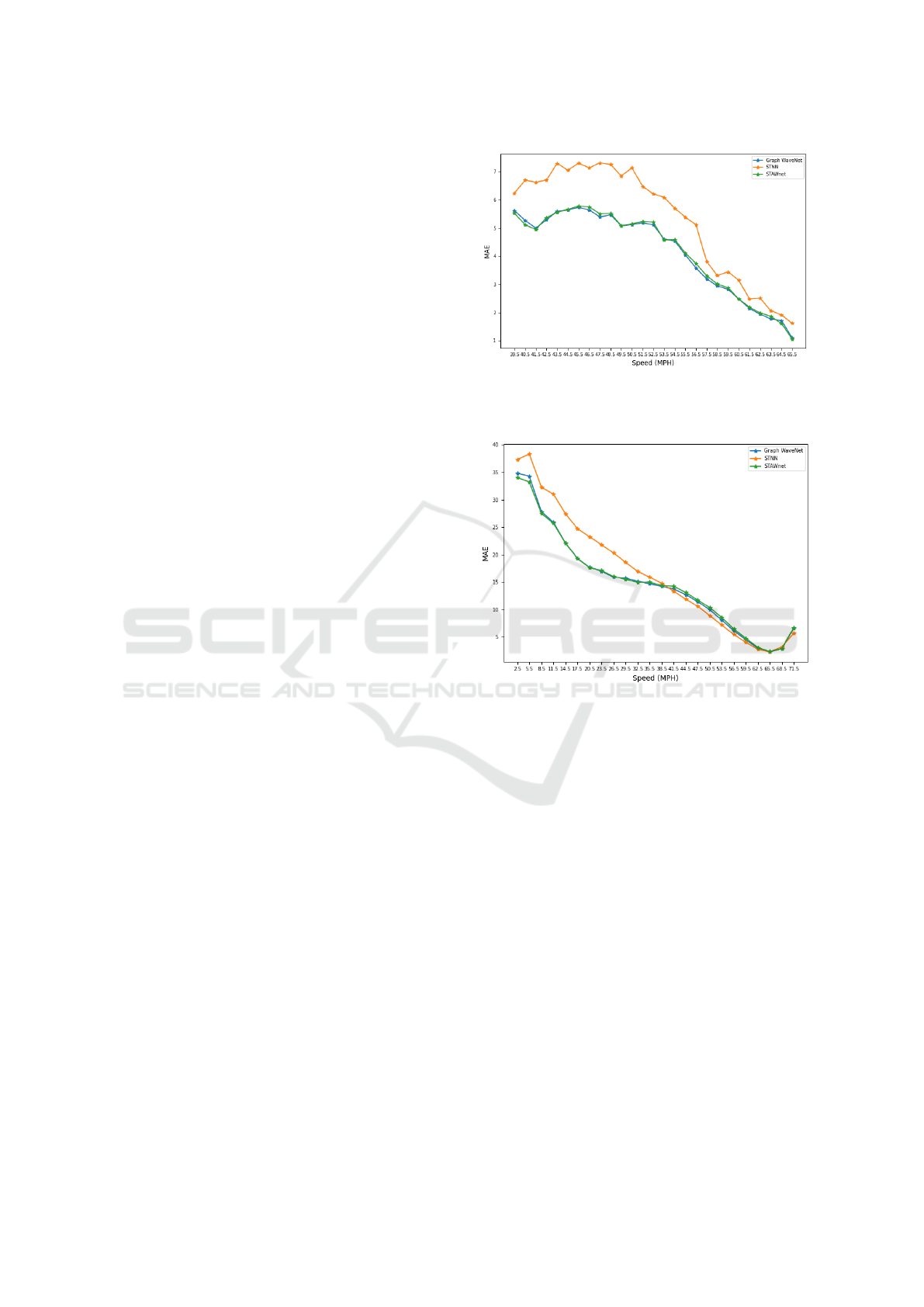
The performance of the three analysed models on

the METR-LA dataset is shown in Fig. 1 for the

Figure 1: Model performance (MAE) for 60 minute predic-

tion horizon, binned per average network speed for METR-

LA test set.

Figure 2: Model performance (MAE) for 60 minute predic-

tion horizon, binned per sensor speeds for METR-LA test

set.

binned average network speed and in Fig. 2 for the

binned sensor speed. As expected, the three models

perform better for faster trafﬁc speeds and worse for

slower trafﬁc speeds. This is an indication of the ex-

tent to which the performance of the trafﬁc forecast-

ing models deteriorates during times of congestion in

the road network. Similar results are observed for the

PeMS-Bay dataset. In both cases, the x ticks indicate

the centre speed value in the bins, and the bins all have

the same sizes.

4.2 Congestion Analysis

All results in this section are reported on the valida-

tion set as we aim to use some of this information

during later congestion modelling. We ﬁrst analyse

network speed averaged across time and day of the

week, to determine the signiﬁcance of recurrent con-

gestion. We then analyse the effect of congestion us-

ing different congestion thresholds and three ways to

NCTA 2022 - 14th International Conference on Neural Computation Theory and Applications

334

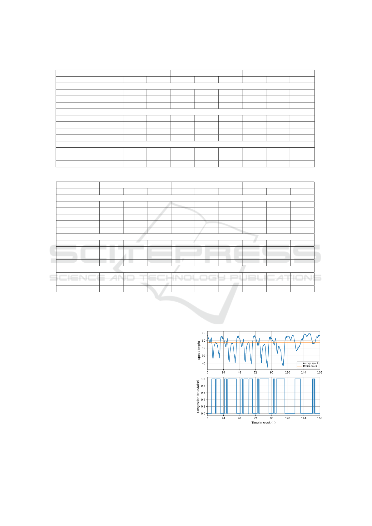
Table 2: Published and recreated performance of selected SOTA trafﬁc speed prediction models: METR-LA, test set.

15 min 30 min 60 min

MAE RMSE MAPE MAE RMSE MAPE MAE RMSE MAPE

Published results

STNN 2.27 4.46 5.80% 2.56 5.29 6.84% 3.01 6.23 8.50%

STAWnet 2.70 5.22 6.98% 3.04 6.14 8.22% 3.44 7.16 9.82%

Graph WaveNet 2.69 5.15 6.90% 3.07 6.22 8.37% 3.53 7.37 10.01%

Recreated results

STNN 2.29 4.45 5.80% 2.59 5.22 6.84% 3.03 6.26 8.94%

STAWnet 2.72 5.26 6.97% 3.08 6.22 8.30% 3.50 7.27 9.96%

Graph WaveNet 2.69 5.13 6.76% 3.05 6.12 8.17% 3.49 7.21 9.82%

STNN adjusted 2.67 5.28 7.31% 3.19 6.47 9.21% 3.96 8.01 12.34%

Difference between published and recreated results

STNN -0.88% 0.22% 0.00% -1.17% 1.32% 0.00% -0.66% -0.48% 0.12%

STAWnet -0.74% -0.77% 0.14% -1.32% -1.30% -0.97% -1.74% -1.54% -1.43%

Graph WaveNet 0.00% 0.38% 2.03% 0.65% 1.61% 2.39% 1.13% 2.17% 1.89%

Table 3: Published and recreated performance of selected SOTA trafﬁc speed prediction models: PeMS-Bay, test set.

15 min 30 min 60 min

MAE RMSE MAPE MAE RMSE MAPE MAE RMSE MAPE

Published results

STNN 1.20 2.41 2.53% 1.50 3.26 3.33% 1.86 4.22 4.30%

GMAN 1.34 2.82 2.81% 1.62 3.72 3.63% 1.86 4.32 4.31%

STAWnet 1.31 2.78 2.76% 1.62 3.70 3.67% 1.89 4.36 4.47%

Graph WaveNet 1.30 2.74 2.76% 1.63 3.70 3.67% 1.95 4.52 4.63%

STTN 1.36 2.87 2.89% 1.67 3.79 3.78% 1.95 4.50 4.58%

Recreated results

STNN 1.21 2.43 2.51% 1.49 3.23 3.23% 1.87 4.18 4.32%

STAWnet 1.32 2.81 2.77% 1.64 3.75 3.69% 1.95 4.46 4.52%

Graph WaveNet 1.30 2.72 2.71% 1.62 3.66 3.64% 1.93 4.43 4.52%

STNN adjusted 1.41 2.94 2.96% 1.83 4.09 4.25% 2.35 5.27 5.85%

Difference between published and recreated results

STNN -0.83% -0.83% 0.79% 0.67% 0.92% 3.00% -0.54% 0.95% -0.47%

STAWnet -0.76% -1.08% -0.36% -1.24% -1.35% -0.55% -3.18% -2.29% -1.12%

Graph WaveNet 0.00% 0.73% 1.81% 0.61% 1.08% 0.82% 1.03% 1.99% 2.38%

combine predictions: average network speed, recur-

rent congestion across all days, and recurrent conges-

tion excluding weekends. Finally, we demonstrate the

effect of congestion as the prediction horizon is var-

ied.

In Fig. 3 we show the recurrent congestion ob-

served in the METR-LA data set. The ﬁrst 120 hours

represent the average network speed Monday to Fri-

day and the remaining period represents the weekend.

There is a clear drop in average network speed during

certain intervals of a typical day. These intervals are

also more prominent during weekdays (referred to as

‘work days’ for clarity). These intervals can be de-

scribed as periods of congestion. To select periods of

congestion for analysis, we can use a threshold, such

as the median trafﬁc speed used in Fig. 3, to separate

the congested and not congested data.

To compare model performance during times of

congestion with performance during the absence of

congestion, we set different congestion thresholds

around the median speed measured across all sensors,

computed using the training partition of the METR-

LA and PeMS-Bay datasets. We start with a thresh-

old value that equals the median speed over all sensors

and then vary this threshold, to obtain different divi-

Figure 3: METR-LA training set average network speed per

time of day and day of week, and matching congested inter-

vals.

A Comparative Study of Graph Neural Network Speed Prediction during Periods of Congestion

335

sions of the data set, by adding or subtracting a thresh-

old interval value. We use two different size intervals

for speeds faster and slower than the median thresh-

old, as the data distribution is skewed. The threshold

values that are smaller than the median speed are de-

termined by subtracting multiples of a threshold in-

terval value computed using Eq. 4 from the median

speed, while the thresholds that are larger than the

median speed are calculated by adding multiples of

the interval value calculated using Eq. 5 to the me-

dian speed value.

− min(s)

(4)

max(s) − s

(5)

In Eq. 4 and 5 s is the average network speed

(across all sensors, per time step), s

is the centre

threshold speed (in this case the median), and s

and

are the speed intervals, slower and faster than the

median, respectively.

For our ﬁrst analysis, we compare the average net-

work speed at each time step in the validation set to

the threshold speed. If the average network speed is

greater than the threshold speed, the network at this

time step is not congested, otherwise, the network

is congested. The prediction MAE during congested

times is then compared to the prediction MAE dur-

ing not congested times across the entire validation

set and the complete trafﬁc network. Fig. 4

depicts the following for Graph WaveNet for dif-

ferent threshold values: the number of observations

that form part of the congested and not congested

data, the average MAE for the 60-minute prediction

horizon for congested and not congested data, and the

difference in MAE between the predictions for con-

gested values and not congested data. From these re-

sults the difference in the performance of the models

for congested data and not congested data is clear.

For our second analysis, we use a ﬁxed daily di-

vision between congested and not congested data by

calculating the average daily speed over all days for

each time of day. The threshold value is then com-

pared with this ﬁxed daily average speed pattern to

differentiate between congested and not congested

observations. As each prediction uses the past hour

of measured speeds, the daily time interval that repre-

sents times of recurrent congestion is chosen as from

the hour before the average daily speed drops below

the threshold until the hour before the average daily

speed goes above the threshold for the last time in the

training dataset. This time interval of data is then ex-

tracted from the dataset as the congested data and the

Figure 4: Graph WaveNet per time-step congestion analy-

sis: METR-LA, validation set.

rest of the data is the not congested data. The perfor-

mance of the model during the congested time inter-

val is then compared to the performance of the model

outside of this interval. For the third analysis we use

the same method as for the second analysis to deter-

mine recurrent daily congestion patterns, but exclude

weekend data.

The result for the three described analyses are

given in Table 4 for the METR-LA dataset and in Ta-

ble 5 for the PeMS-Bay dataset. The median thresh-

old is indicated in bold along with the maximum

MAE differences. By examining the results in Tables

4 and 5 we can see that STNN does not generalise as

well as STAWnet and Graph WaveNet on congested

data since the difference in performance on congested

and not congested data is much larger for STNN than

it is for the other two models. We can also see that, by

excluding weekend data from the recurrent conges-

tion analysis, a bigger difference is obtained in per-

formance on congested and not congested data. This

is because, as can be seen in Fig. 3, weekend data has

a smaller interval of congestion during the day and

the same recurrent congestion interval can therefore

not effectively be used for weekends.

Finally, we consider the interplay between con-

gestion and the prediction horizon. In Fig. 5 we show

the performance of the METR-LA Graph WaveNet

model when categorising congestion data based on

average network speed per time step and using the

median as a threshold. Not only is the model’s per-

formance worse for data above the threshold, but the

performance of the model also becomes worse more

rapidly with increasing prediction horizons. This is a

clear indication of how improving the model’s perfor-

mance during times of congestion would beneﬁt the

model’s trafﬁc prediction capabilities.

NCTA 2022 - 14th International Conference on Neural Computation Theory and Applications

336

Table 4: Performance of the selected systems when evaluated using the three congestion scenarios: The MAE on congested

data, and the MAE difference when evaluated on congested and not congested data as the congestion threshold is varied.

METR-LA, validation set, 60-min horizon.

Threshold (MPH) 50.97 51.94 52.90 53.86 54.83 57.72 58.22 58.72 59.21 59.71

MAE per time step

GWN congested 5.75 5.68 5.68 5.62 5.52 4.98 4.85 4.76 4.66 4.54

GWN difference 3.07 3.06 3.12 3.13 3.11 2.78 2.69 2.64 2.59 2.52

STNN congested 7.57 7.52 7.46 7.33 7.11 5.99 5.88 5.80 5.70 5.54

STNN difference 4.46 4.47 4.48 4.44 4.31 3.41 3.35 3.31 3.24 3.13

STAWnet congested 5.72 5.66 5.67 5.63 5.52 5.00 4.89 4.80 4.70 4.57

STAWnet difference 2.99 2.98 3.07 3.09 3.06 2.76 2.69 2.63 2.58 2.50

MAE recurrent congestion: all days

GWN congested 4.38 4.40 3.87 3.87 3.87 3.88 3.88 3.55 3.54 3.53

GWN difference 1.34 1.43 1.29 1.36 1.39 1.50 1.51 1.21 1.24 1.25

STNN congested 5.44 5.47 4.45 4.49 4.51 4.55 4.55 4.15 4.13 4.12

STNN difference 1.92 2.04 1.39 1.55 1.61 1.80 1.82 1.45 1.48 1.50

STAWnet congested 4.43 4.43 3.90 3.89 3.89 3.91 3.91 3.59 3.57 3.57

STAWnet difference 1.35 1.41 1.27 1.32 1.35 1.49 1.50 1.18 1.21 1.23

MAE recurrent congestion: work days only

GWN congested 5.05 5.16 4.54 4.55 4.57 4.60 4.60 4.15 4.14 4.13

GWN difference 1.62 1.83 1.74 1.85 1.91 2.11 2.13 1.71 1.76 1.79

STNN congested 6.41 6.51 5.21 5.31 5.35 5.43 5.44 4.88 4.86 4.85

STNN difference 2.39 2.62 1.81 2.08 2.19 2.50 2.53 2.05 2.10 2.14

STAWnet congested 5.10 5.18 4.58 4.60 4.61 4.65 4.65 4.19 4.18 4.17

STAWnet difference 1.62 1.79 1.73 1.84 1.89 2.11 2.13 1.69 1.73 1.76

Table 5: Same analysis as in Table 4 but for the PeMS-Bay task.

Threshold (MPH) 57.42 58.44 59.47 60.49 61.51 62.53 63.55 63.92 64.28 64.64

MAE per time stem

GWN congested 3.70 3.68 3.66 3.62 3.52 3.25 2.90 2.84 2.80 2.76

GWN difference 2.28 2.31 2.34 2.35 2.30 2.12 1.83 1.78 1.75 1.73

STNN congested 5.41 5.39 5.35 5.29 5.12 4.64 4.09 3.99 3.93 3.88

STNN difference 3.64 3.70 3.74 3.75 3.66 3.28 2.81 2.74 2.70 2.67

STAWnet congested 3.76 3.74 3.70 3.66 3.55 3.28 2.93 2.86 2.82 2.78

STAWnet difference 2.34 2.36 2.38 2.37 2.32 2.12 1.83 1.79 1.75 1.73

MAE recurrent congestion all days

GWN congested 2.63 2.66 2.67 2.68 2.68 2.67 2.64 2.63 2.61 2.60

GWN difference 1.24 1.37 1.42 1.49 1.54 1.59 1.60 1.61 1.61 1.61

STNN congested 3.49 3.61 3.63 3.67 3.70 3.71 3.69 3.68 3.65 3.63

STNN difference 1.60 1.90 1.99 2.13 2.28 2.41 2.47 2.48 2.48 2.48

STAWnet congested 2.66 2.70 2.70 2.71 2.71 2.69 2.67 2.66 2.63 2.62

STAWnet difference 1.27 1.40 1.44 1.51 1.56 1.60 1.61 1.62 1.61 1.61

MAE recurrent congestion work days

GWN congested 2.96 3.01 3.03 3.05 3.05 3.04 3.01 3.00 2.98 2.96

GWN difference 1.45 1.62 1.68 1.78 1.85 1.91 1.94 1.95 1.95 1.95

STNN congested 3.99 4.15 4.19 4.24 4.29 4.31 4.29 4.28 4.24 4.22

STNN difference 1.85 2.25 2.37 2.56 2.75 2.93 3.02 3.04 3.04 3.04

STAWnet congested 3.00 3.06 3.07 3.08 3.08 3.07 3.04 3.03 3.00 2.99

STAWnet difference 1.48 1.66 1.71 1.80 1.87 1.93 1.95 1.96 1.95 1.95

5 CONCLUSION

In this paper, we investigated the performance of deep

learning models for trafﬁc speed prediction during pe-

riods of congestion. We found that, while all the

techniques investigated performed similarly in the ab-

sence of congestion, Graph WaveNet and STAWnet

outperformed STNN during periods of congestion. It

was also found that a longer prediction horizon had a

large effect on performance during periods of conges-

tion, and a surprisingly limited effect otherwise. An

increased understanding of model behaviour during

congestion should assist future efforts to optimise a

model for periods of recurrent congestion, which will

improve route-ﬁnding algorithms during times of the

day when fastest path-ﬁnding technologies are most

necessary. An increase in a model’s ability to accu-

rately predict trafﬁc during recurrent congestion will

A Comparative Study of Graph Neural Network Speed Prediction during Periods of Congestion

337

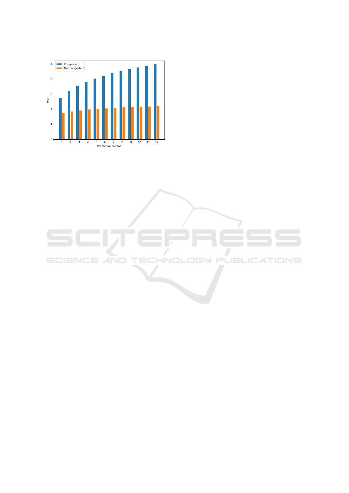
Figure 5: Graph WaveNet per time-step performance on

METR-LA dataset for data above and below the median

congestion threshold for twelve prediction horizons.

most likely also increase its performance during non-

recurrent congestion events such as trafﬁc accidents.

Future work will focus on improving prediction

performance during periods of congestion. To opti-

mise a trafﬁc speed prediction model’s performance

during times of congestion, segments of the day that

represent recurrent congestion can be extracted and

used to train the model and congestion data can also

be repeated within the training set. The loss function

of the model can also be modiﬁed to give preference

to congestion data during training. This will be ex-

plored in future work.

REFERENCES

Akhtar, M. and Moridpour, S. (2021). A review of traf-

ﬁc congestion prediction using artiﬁcial intelligence.

Journal of Advanced Transportation, 2021:1–18.

Chikaraishi, M., Garg, P., Varghese, V., Yoshizoe, K., Urata,

J., Shiomi, Y., and Watanabe, R. (2020). On the pos-

sibility of short-term trafﬁc prediction during disas-

ter with machine learning approaches: An exploratory

analysis. Transport Policy, 98:91–104.

Gandhi, M. M., Solanki, D. S., Daptardar, R. S., and

Baloorkar, N. S. (2020). Smart control of trafﬁc light

using artiﬁcial intelligence. In Proc. IEEE Int. Conf.

on Recent Advances and Innovations in Engineering

(ICRAIE), pages 1–6.

Gunawan, F. E. and Chandra, F. Y. (2014). Optimal averag-

ing time for predicting trafﬁc velocity using ﬂoating

car data technique for advanced traveler information

system. Procedia - Social and Behavioral Sciences,

138:566–575. The 9th Int. Conf. on Trafﬁc and Trans-

portation Studies (ICTTS).

Jiang, Z., Guo, F., Qian, Y., Wang, Y., and Pan, W. D.

(2021). A deep learning-assisted mathematical model

for decongestion time prediction at railroad grade

crossings. Neural Computing and Applications, page

4715–4732.

Li, Y., Yu, R., Shahabi, C., and Liu, Y. (2018). Diffusion

convolutional recurrent neural network: Data-driven

trafﬁc forecasting. In Int. Conf. on Learning Repre-

sentations.

Mallick, T., Balaprakash, P., Rask, E., and Macfarlane,

J. (2020). Transfer learning with graph neural net-

works for short-term highway trafﬁc forecasting. In

Proc. Int. Conf. on Pattern Recognition (ICPR), pages

10367–10374.

Mena-Oreja, J. and Gozalvez, J. (2020). A comprehensive

evaluation of deep learning-based techniques for traf-

ﬁc prediction. IEEE Access, 8:91188–91212.

Mohanty, S. (2018). A Deep Learning, Model-Predictive

Approach to Neighborhood Congestion Prediction

and Control. PhD thesis, Berkeley University of Cal-

ifornia.

Nagy, A. M. and Simon, V. (2018). Survey on trafﬁc predic-

tion in smart cities. Pervasive and Mobile Computing,

50:148–163.

Polson, N. G. and Sokolov, V. O. (2017). Deep learning

for short-term trafﬁc ﬂow prediction. Transportation

Research Part C: Emerging Technologies, 79:1–17.

Shi, G., Shan, J., Ding, L., Ye, P., Li, Y., and Jiang, N.

(2019). Urban road network expansion and its driving

variables: A case study of Nanjing City. Int. Jour-

nal of Environmental Research and Public Health,

16:2318–2334.

Tian, C. and Chan, W. K. V. (2021). Spatial-temporal atten-

tion wavenet: A deep learning framework for trafﬁc

prediction considering spatial-temporal dependencies.

IET Intelligent Transport Systems, 15:549–561.

Wu, Z., Pan, S., Long, G., Jiang, J., and Zhang, C. (2019).

Graph WaveNet for deep spatial-temporal graph mod-

eling. In Proc. of the 28th Int. Joint Conf. on AI,

IJCAI-19, pages 1907–1913.

Xu, J., Zhang, Y., and Xing, C. (2018). An effective selec-

tion method for vehicle alternative route under traf-

ﬁc congestion. In Proc. Int. Conf. on Communication

Technology (ICCT), pages 494–499.

Xu, M., Dai, W., Liu, C., Gao, X., Lin, W., Qi, G.-

J., and Xiong, H. (2020). Spatial-temporal trans-

former networks for trafﬁc ﬂow forecasting. ArXiv,

abs/2001.02908.

Yang, S., Liu, J., and Zhao, K. (2021). Space meets time:

Local spacetime neural network for trafﬁc ﬂow fore-

casting. In Proc. IEEE Int. Conf. on Data Mining

(ICDM), pages 817–826.

Zheng, C., Fan, X., Wang, C., and Qi, J. (2020). GMAN: A

graph multi-attention network for trafﬁc prediction. In

Proc. AAAI Conf. on AI, volume 34, page 1234–1241.

Zhou, L., Zhang, S., Yu, J., and Chen, X. (2020).

Spatial–temporal deep tensor neural networks for

large-scale urban network speed prediction. IEEE

Transactions on Intelligent Transportation Systems,

21(9):3718–3729.

Zliobait

e, I. and Khokhlov, M. (2016). Optimal estimates

for short horizon travel time prediction in urban areas.

Intelligent Data Analysis, 20(6):1459–1475.

NCTA 2022 - 14th International Conference on Neural Computation Theory and Applications

338