Application of Data-driven Deep Learning Model in Global

Precipitation Forecasting

Wan Liu

1,2

and Yongqiang Wang

1,2

Changjiang River Scientific Research Institute of Changjiang Water Resources Commission,

23 Huangpu Street, Wuhan, China

Hubei Provincial Key Laboratory of Basin Water Resources and Ecological Environment,

23 Huangpu Street, Wuhan, China

Keywords: Precipitation Forecasting, Deep Learning, ConvLSTM, ConvGRU.

Abstract: With the improvement of data acquisition ability and the rapid increase of computer storage capacity and

transmission rate, it is possible to solve the problem of precipitation prediction by using big data and deep

learning. In this paper, the three most advanced deep learning models, namely Convolution model,

ConvLSTM model and ConvGRU model, are applied to the study of precipitation prediction, and analyze the

prediction ability of this method for global short-term precipitation. The experimental results show that the

deep learning method can effectively predict global precipitation, and the correlation coefficient of

precipitation prediction for the next 6 h is more than 0.75. The performance of convolution model is better

when the prediction period is less than 12 h, Otherwise ConvLSTM model and ConvGRU model are more

efficient. However, it is difficult to predict precipitation over northern Africa, the west coast of South

America, the eastern coast of the South Pacific and the South Atlantic.

1 INTRODUCTION

Precipitation has a great impact on human production

and social development. In addition, precipitation is

an important part of water resources ecosystem, and

plays an important role in hydrology, meteorology,

and other aspects. Short-term heavy rainfall is prone

to flood, mudslides, urban waterlogging, and other

disasters, resulting in casualties and property losses.

Therefore, it is of great significance to forecast

precipitation, especially extreme rainfall.

Precipitation is the result of the interaction of multi-

scale air system, which is affected by a variety of

environmental factors. These complex physical

mechanisms make it very difficult to predict

precipitation (Tran, 2019, Song, 2019). At present,

numerical model prediction (Simonin, et al., 2017,

Bauer, et al., 2015) and echo extrapolation (Wang, et

al., 2013, Ayzel, et al., 2019b) are the most

commonly used methods in precipitation prediction.

However, both have certain limitations for short-term

forecasting (Bližňák, et al., 2017). Therefore, due to

the complex dynamic changes of the atmosphere and

the real-time requirements of short-term precipitation

forecast, large-scale and high-precision forecast

models are urgently needed, which poses great

challenges to the fields of meteorology and

hydrology.

With the development of satellite and radar

detection technology, a mass of earth system data can

be obtained. Meanwhile, the rapid increase of

computer storage capacity and transmission rate

makes it possible to use big data and deep learning to

solve the problem of short impending precipitation

prediction (Song, et al., 2019, Su, et al., 2020, Qiu, et

al., 2017). As a kind of nonlinear mathematical model

driven by data, deep learning technology has

excellent feature learning ability (Reichstein, et al.,

2019). It can automatically learn massive data,

consequently mine the inherent characteristics of data

and the inherent physical laws. For the complex

spatio-temporal dynamic system, without a complete

understanding of its internal mechanism, the

nonlinear characteristics of the complex atmospheric

can be characterized by learning historical data

through machine learning method even without using

the mathematical and physical equations controlling

the atmosphere. In recent years, artificial intelligence

technology represented by deep learning has made

major breakthroughs in image recognition,

318

Liu, W. and Wang, Y.

Application of Data-driven Deep Learning Model in Global Precipitation Forecasting.

DOI: 10.5220/0011176400003440

In Proceedings of the International Conference on Big Data Economy and Digital Management (BDEDM 2022), pages 318-324

ISBN: 978-989-758-593-7

nowcasting and other fields, and even surpassed the

level of human intelligence in some tasks (LeCun, et

al., 2015).

Precipitation forecast can be regarded as a spatio-

temporal series prediction problem, which is to

predict the spatial distribution of precipitation in the

future on the premise of knowing the continuous

spatial distribution of some variables in the past

period (Shi, et al., 2015). Therefore, Recurrent neural

network (RNN) (Wang, et al., 2021) which is good at

learning temporal features of data, and Convolutional

neural network (CNN) (Ayzel, et al., 2019a) which is

good at extracting spatial features of data, are often

used to study short-term precipitation forecast. (Klein

et al., 2015) present Dynamic Convolutional Layer,

which is a generalization of convolutional layer, and

apply it to short range weather prediction. (Wang, et

al. 2018) proposed a Memory in Memory (MIM)

network for precipitation nowcasting. (Shi, et al.,

2015) combined CNN and RNN for the first time and

proposed a convolutional long short-term memory

(ConvLSTM) model to perform precipitation

nowcasting. Subsequently, (Shi, et al., 2017) further

proposed Trajectory Gated Recurrent Unit

(TrajGRU) model, which is more effective than

Convolutional Gated Recurrent Unit (ConvGRU)

(Ballas et al., 2015) in capturing temporal and spatial

correlation. (Tian, et al., 2020) proposed a generative

adversarial ConvGRU (GA-ConvGRU) model,

which significantly outperforms ConvGRU.

In this work, we apply the deep learning model to

the precipitation prediction project, using the most

advanced convolution model, ConvLSTM model and

ConvGRU model to achieve global precipitation

forecast. Analyse and compare the advantages and

disadvantages of the three models, and test their

forecasting ability in different regions of the world.

2 MATERIALS AND METHODS

2.1 Data Collection and Pre-processing

The data used in this study are NCEP FNL

Operational Global Analysis Data from 2015-2021,

which is a global reanalysis data jointly produced by

National Center for Environmental Prediction

(NCEP) and National Center for Atmospheric

Research (NCAR). These data are from the Global

Data Assimilation System (GDAS), which

continuously collects observational data from the

Global Telecommunications System (GTS), and

other sources, for many analyses. These data are on

1-degree by 1-degree grids prepared operationally

every six hours.

We selected four meteorological variables

associated with precipitation as predictors of the

model, which are relative humidity (x

), temperature

), radial wind speed (x

) and zonal wind speed (x

)

at 500 hPa height. Precipitation systems are often

controlled by weather systems of 500 hPa. Relative

humidity represents the moisture content of the

precipitation system and is the most basic condition

for the occurrence of precipitation. Temperature

affects the internal energy of a precipitation system.

Radial wind speed and zonal wind speed affects the

direction and speed of precipitation system

movement.

Data preprocessing is required for the predictors

to be able to enter the model and predict precipitation

effectively. Firstly, to save the training and prediction

time of the model, the spatial resolution of the data

including the predictors and precipitation data was

compressed to 2 degrees. As the units and orders of

magnitude of each predictor are different, data need

to be normalized to achieve a unified dimension,

cancel the difference of orders of magnitude between

data, and avoid large network prediction errors

caused by large difference of orders of magnitude

between input and output data. One of the most

commonly used data normalization methods is min-

max normalization. It standardizes the data to

between 0 and 1. The normalization formula of min-

max is as follows:

min

max min

−

(1)

Where, x represents a value in the sequence of

primitive variables, x* represents the normalized

value of x, x

max

and x

min

represent the maximum and

minimum values in variables, respectively.

Subsequently, all predictors at the same time were

spliced together to form a tensor X with a size of (90,

180, 4). Data were sampled according to the time

sequence to obtain the input samples {X

t-7

, …, X

t-1

} at time t, where X

t-1

and X

are a group of

predictors with a time interval of 6 hours. Similarly,

sample output {Y

, Y

t+1

, Y

t+2

, Y

t+3

} corresponding to

sample input at time t can be obtained, where Y

is the

precipitation in the next 6 hours starting from time t.

2.2 Deep Learning Model for

Precipitation Forecasting

Deep learning methods for precipitation forecasting

usually need to consider the temporal and spatial

Application of Data-driven Deep Learning Model in Global Precipitation Forecasting

319

correlation of data, therefore the commonly used

models are Convolution model, ConvLSTM model

and ConvGRU model. From the spatial viewpoint, P

observations of weather system at same time over a

spatial region with an M × N grid can be treated as a

tensor x∈R

P×M×N

. From the temporal viewpoint, a

sequence of tensors x

, x

, ..., x

can be obtained by

collecting observations at fixed time intervals over

time. Thus, this precipitation nowcasting problem can

be illustrated as:



()

...

,..., ... ...

ttL

ttLt-K+1 t

Y, ,Y

Y = argmax p Y , ,Y X , XY,

∣

(2)

Where, {X

t-K+1

, ..., X

} is the historical observation

sequence data of length K, and {Y

, ..., Y

t+L

} is the

predicted precipitation sequence data of length L in

the future.

For Convolution model, since the 2D convolution

model cannot capture the information on the time

sequence well, the 3D convolution model is adopted.

Model regards the time dimension as the third

dimension and forms a cube by stacking multiple

consecutive frames to calculate the 3D convolution in

the cube. The 3D convolution formula is as follows:

()YWXb

=∗+

(3)

Where,

represents the Sigmoid activation

function, W represents the convolution kernel, *

represents the convolution operator, and b represents

the offset.

ConvLSTM model, Shi et al proposed, combines

convolutional neural network with LSTM to

determine the future state of a cell by its adjacent

input units and past states. The input in LSTM model

is extended to three dimensions, and the state-to-state

and input-to-state are realized by convolution layer.

The calculation formula of ConvLSTM is as follows:

()

tanh( )

txithitciti

txfthftcftf

txothotcoto

ttt t xct hct c

tt t

iWxWhWcb

fWxWhWcb

oWxWhWcb

cfc i WxWh b

ho c

−−

=∗+∗+ +

=+ ∗+∗+







(4)

Where, x

, h

and c

represent the inputs, hidden

states, and unit outputs respectively, i

, f

and o

represent the three gate controls, and ° represents the

Hadamard product.

ConvGRU network is ConvLSTM network

variant. ConvGRU has fewer parameters and faster

training convergence time than ConvLSTM, because

ConvGRU controls the information flow and

removes the memory unit by two gates, the update

and reset gates, while ConvLSTM has three gates.

The main formulas are given as follows:

()

-1

txzthzt

txrthrt

txhtthht

ttttt

zsWxWh

rsW xWh

hfWxrWh

hzhzh

=+°

=°+°

(5)

Where, f is the activation function, h

, z

, r

, and h

’

are the memory state, update gate, reset gate, and new

information, respectively. The reset gate is used to

control the previous timestamp state h

t-1

into the

ConvGRU. The update gate controls the extent to

which the previous timestamp state h

t-1

and the new

input h

’ affect the new state vector h

2.3 Model Structure

The model structure includes three parts: data

dimension reduction, sequence prediction and feature

reconstruction. Firstly, there are three convolution

layers, each of which has 16, 32, 32 convolution

kernels respectively. The maximum pooling layers

are added after the last two convolution layers to

reduce data dimension. The sequence prediction part

has 6 layers, and each layer has 64 convolution

kernels. For the convolution model, layers are

convolution networks. For ConvLSTM and

ConvGRU, the ConvLSTM networks or ConvGRU

networks. Finally, there are 4 convolution layers,

with 32, 16, 3 and 1 convolution kernel respectively.

Upsampling layers are added after the first two

convolution layers to restore the data. In addition,

batch normalization layer (BN) was added after each

convolutional layer and ConvLSTM layer to speed up

the training process and improve performance. The

size of all 3D convolution kernels in the model is

(3,3,3). The convolution kernels of ConvLSTM and

ConvGRU are (5,5). The model structure of

ConvLSTM model is shown in Figure 1.

BDEDM 2022 - The International Conference on Big Data Economy and Digital Management

320

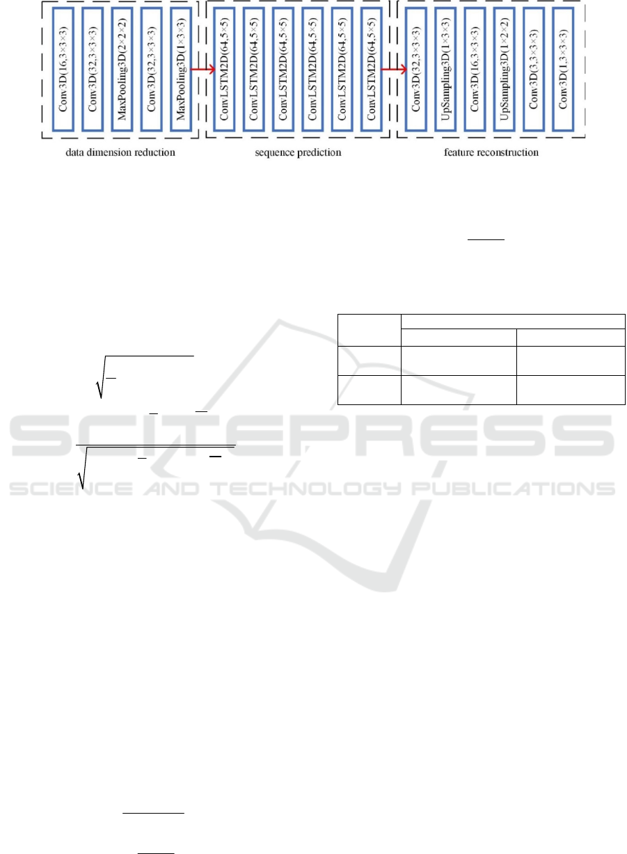
Figure 1: The model structure of ConvLSTM model.

3 EXPERIMENTS

3.1 Evaluation Methods

In this paper, we use root mean square error (RMSE)

and correlation coefficient (CC) to evaluate the

accuracy of the model. The calculation formula of

RMSE and correlation coefficient is as follows:

()

RMSE y y

=−



)

2''2

()( )

yyyy

yy yy

−−





)

Where, y

and y

' are measured value and model

predicted value respectively, ⎯y and ⎯y' are measured

average value and model predicted average value

respectively, and n is the number of samples. The

larger CC value is, the higher the positive correlation

between y and y' is, the better the prediction effect is.

In addition, to analyze the impact of the model on

rainstorm forecast, a precipitation threshold k was set,

and the samples were classified according to the

relationship among observed precipitation, predicted

precipitation and threshold, as shown in Table 1.

According to the successful prediction times (A),

empty prediction times (B) and prediction failure

times (C), the commonly used evaluation indexes of

precipitation prediction such as critical success index

(CSI), false alarm rate (FAR) and probability of

detection (POD) were obtained to evaluate the effect

of the model. The calculation formula of CSI, FAR

and POD is as follows:

CSI

(8)

FAR

(9)

POD

(10)

Table 1: Test index classification table of precipitation

nowcasting.

Observed

Value

redicted value

≥

k <k

≥k

A (successful

rediction

)

C (missed

rediction

)

B (empty

rediction)

D (invalid data)

3.2 Results

We chose three deep learning models to conduct

precipitation prediction experiments, namely,

convolution model, ConvLSTM model and

ConvGRU model. The RMSE and CC of the

predicted results are shown in Table 2. Set the

threshold value k = 0.5 mm and k = 3 mm to calculate

the evaluation indexes of precipitation forecast,

including CSI, FAR and POD. The results are shown

in Table 3.

As shown in Table 2, the application of deep

learning model to precipitation forecast projects can

achieve good performance, and the forecast accuracy

will decrease with the increase of forecast period.

Correlation coefficient of results in the first 6 hours

are all greater than 0.75 and RMSE are all less than

1.395 mm. The RMSE and CC of the ConvLSTM and

ConvGRU models are always very similar,

nevertheless the ConvGRU model had fewer

parameters and faster training and prediction times.

When the prediction period is less than 12 h, the

performance of the convolution model is the best.

While the prediction period is more than 12 h,

ConvLSTM and ConvGRU models are superior to

Convolution model due to the weak time correlation

extraction ability of the Convolution model.

Application of Data-driven Deep Learning Model in Global Precipitation Forecasting

321

Table 2: The RMSE and CC of the predicted results.

Model

6 h 12 h 18 h 24 h

RMSE CC RMSE CC RMSE CC RMSE CC

Convolution model 1.345

0.785 1.389 0.750 1.448 0.697 1.492 0.648

ConvLSTM model

1.384 0.755 1.401 0.742 1.428 0.713 1.459 0.683

ConvGRU model

1.395 0.750 1.405 0.740 1.431 0.717 1.461 0.685

Table 3: The evaluation indexes of predicted results.

Model

k = 0.5 mm k = 3 mm

CSI FAR CSI FAR CSI FAR

Convolution model 0.546

0.402 0.546 0.402 0.546 0.402

ConvLSTM model

0.576 0.335 0.576 0.335 0.576 0.335

ConvGRU model

0.572 0.327 0.572 0.327 0.572 0.327

We chose three deep learning models to conduct

precipitation prediction experiments, namely,

convolution model, ConvLSTM model and

ConvGRU model. The RMSE and CC of the

predicted results are shown in Table 2. Set the

threshold value k = 0.5 mm and k = 3 mm to calculate

the evaluation indexes of precipitation forecast,

including CSI, FAR and POD. The results are shown

in Table 3.

As shown in Table 2, the application of deep

learning model to precipitation forecast projects can

achieve good performance, and the forecast accuracy

will decrease with the increase of forecast period.

Correlation coefficient of results in the first 6 hours

are all greater than 0.75 and RMSE are all less than

1.395 mm. The RMSE and CC of the ConvLSTM and

ConvGRU models are always very similar,

nevertheless the ConvGRU model had fewer

parameters and faster training and prediction times.

When the prediction period is less than 12 h, the

performance of the convolution model is the best.

While the prediction period is more than 12 h,

ConvLSTM and ConvGRU models are superior to

Convolution model due to the weak time correlation

extraction ability of the Convolution model.

As shown in Table 3, when k = 0.5 mm, the

evaluation index scores of the three deep learning

models have their own advantages and disadvantages.

The highest CSI score of ConvLSTM model is 0.576,

the lowest FAR score of ConvGRU model is 0.327,

and the highest POD score of Convolution model is

0.863. The POD scores of the three models are all

higher than 0.8, but the CSI scores are only slightly

higher than 0.5, indicating that the missed times of

the model are far less than the number of successful

predictions and the number of empty predictions.

When k = 3 mm, the performance of evaluation

indexes of each model decreased significantly,

especially POD scores.

To further analyze the forecasting ability of the

deep learning model for global precipitation, the

precipitation data was compressed again and the

correlation coefficients of the forecast results at each

grid were calculated respectively, shown in Figure 2.

Overall, the correlation coefficients in most regions

of the world are above 0.75, particularly in 30°S-60°S

and the West Pacific coast. However, the prediction

effect is very poor in part of the areas, and even the

correlation coefficient is less than zero, such as the

Antarctic region, near the equator, northern Africa

and so on.

The Antarctic region has little precipitation due to

low temperatures, and forecasts of precipitation don't

make much sense. The Sahara Desert is located in the

north of Africa, and the special surface conditions

have a great impact on precipitation. However, the

model does not take the surface variables as a

predictor, so the performance of the model in this

region is not good., The conditions that affect

precipitation systems are complex around the equator

so that it’s difficult to predict under global models.

Especially the west coast of South America and the

east coast of the South Pacific exists El Nino

phenomenon. If this area is forecasted separately, the

effect may be improved effectively. In addition, there

is a poor forecast in the east coast of South America,

the southern Atlantic region.

BDEDM 2022 - The International Conference on Big Data Economy and Digital Management

322

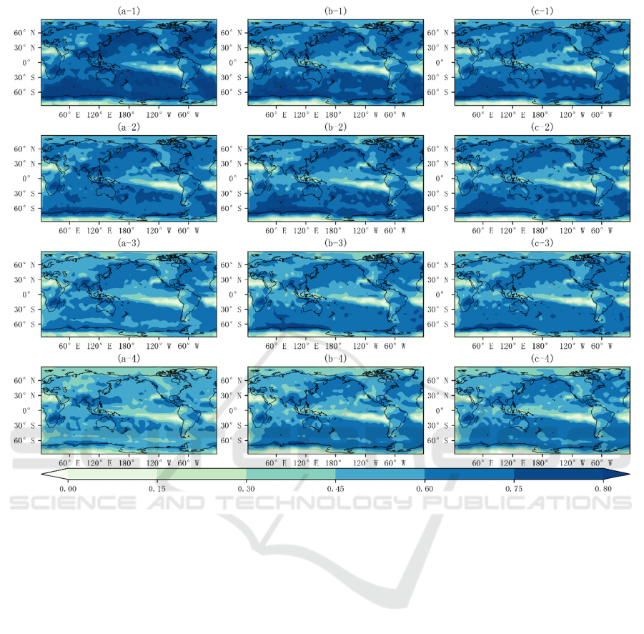
Figure 2: The correlation coefficients of the forecast results at each grid. From left to right, models are (a) Convolution model,

(b)ConvLSTM model, (c)ConvGRU model; from top to bottom, the prediction period are (1) 6 h, (2) 12 h, (3) 18 h, and (4)

24 h.

4 CONCLUSIONS

We introduced the deep learning model into the

precipitation forecast project, using the most

advanced convolution model, ConvLSTM model and

ConvGRU model to achieve global precipitation

forecast. Experimental results show that the overall

forecasting performance of the data-driven method is

excellent. The convolution model has better

prediction results for short-term precipitation.

ConvLSTM and ConvGRU models are more

effective in long-term forecasting. In addition, this

method has strong forecasting ability in 30°S-60°S

and the West Pacific Coast. But in North Africa, the

west coast of South America, the east coast of the

South Pacific, the South Atlantic, this method is

completely unavailable.

In the future, we plan to further study the

application of deep learning in precipitation

prediction and try different network structures and

loss functions to achieve better forecast performance

and faster computational efficiency. Meanwhile, the

study focuses on the influence factors of precipitation

in the west coast of South America, the east coast of

the South Pacific and the South Atlantic region, and

finds out the specific reasons for the difficulty of

forecast in this region, to realize the precipitation

forecast in complex areas.

ACKNOWLEDGEMENTS

This research was financially supported by the Key

Research and Development Program of Ningxia

(2020BCF01002), Water Resource Science and

Application of Data-driven Deep Learning Model in Global Precipitation Forecasting

323

Technology Innovation Program of Guangdong

Province (2017-03), National Natural Science

Foundation of China (51779013, U2040212),

Fundamental Research Funds for Central Public

Welfare Research Institutes (CKSF2021486/SZ,

CKSF2019478/SZ), and National Public Research

Institutes for Basic R & D Operating Expenses

Special Project (CKSF2017061/SZ).

REFERENCES

Ayzel, G., Heistermann, M., Sorokin, A., Nikitin, O. and

Lukyanova, O. (2019a). All convolutional neural

networks for radar-based precipitation nowcasting.

Procedia Computer Science. 150, 186-192.

Ayzel, G., Heistermann, M. and Winterrath, T. (2019b).

Optical flow models as an open benchmark for radar-

based precipitation nowcasting (rainymotion v0.1).

Geoscientific Model Development. 12(4), 1387-1402.

Ballas, N., Yao, L., Pal, C. and Courville, A. (2015).

Delving Deeper into Convolutional Networks for

Learning Video Representations. arXiv:1511.06432.

Bauer, P., Thorpe, A. and Brunet, G. (2015). The quiet

revolution of numerical weather prediction. Nature.

525(7567), 47-55.

Bližňák, V., Sokol, Z. and Zacharov, P. (2017). Nowcasting

of deep convective clouds and heavy precipitation:

Comparison study between NWP model simulation and

extrapolation. Atmospheric Research. 184, 24-34.

Klein, B., Wolf, L. and Afek, Y. 2015. A Dynamic

Convolutional Layer for short rangeweather prediction.

In 2015 IEEE Conference on Computer Vision and

Pattern Recognition (CVPR), pages 4840-4848.

LeCun, Y., Bengio, Y. and Hinton, G. (2015). Deep

learning. Nature. 521(7553), 436-44.

Qiu, M., Zhao, P., Zhang, K., Huang, J., Shi, X., Wang, X.

and Chu, W. 2017. A Short-Term Rainfall Prediction

Model Using Multi-task Convolutional Neural

Networks. In 2017 IEEE International Conference on

Data Mining (ICDM), pages 395-404.

Reichstein, M., Camps-Valls, G., Stevens, B., Jung, M.,

Denzler, J., Carvalhais, N. and Prabhat (2019). Deep

learning and process understanding for data-driven

Earth system science. Nature. 566(7743), 195-204.

Shi, X., Chen, Z., Wang, H., Yeung, D.-Y., Wong, W.-k.

and Woo, W.-c. (2015). Convolutional LSTM

Network: A Machine Learning Approach for

Precipitation Nowcasting. arXiv:1506.04214.

Shi, X., Gao, Z., Lausen, L., Wang, H., Yeung, D.-Y.,

Wong, W.-k. and Woo, W.-c. (2017). Deep Learning

for Precipitation Nowcasting: A Benchmark and A

New Model. arXiv:1706.03458.

Simonin, D., Pierce, C., Roberts, N., Ballard, S. P. and Li,

Z. (2017). Performance of Met Office hourly cycling

NWP-based nowcasting for precipitation forecasts.

Quarterly Journal of the Royal Meteorological Society.

143(708), 2862-2873.

Song, K., Yang, G., Wang, Q., Xu, C., Liu, J., Liu, W., Shi,

C., Wang, Y., Zhang, G., Yu, X., Gu, Z. and Zhang, W.

2019. Deep Learning Prediction of Incoming Rainfalls:

An Operational Service for the City of Beijing China.

In 2019 International Conference on Data Mining

Workshops (ICDMW), pages 180-185.

Su, A., Li, H., Cui, L. and Chen, Y. (2020). A Convection

Nowcasting Method Based on Machine Learning.

Advances in Meteorology. 2020, 1-13.

Tian, L., Li, X., Ye, Y., Xie, P. and Li, Y. 2020. A

Generative Adversarial Gated Recurrent Unit Model

for Precipitation Nowcasting. In IEEE Geoscience

and Remote Sensing Letters, pages 601-605.

Tran, Q.-K. and Song, S.-k. (2019). Computer Vision in

Precipitation Nowcasting: Applying Image Quality

Assessment Metrics for Training Deep Neural

Networks. Atmosphere. 10(5).

Wang, G., Wong, W., Liu, L. and Wang, H. (2013).

Application of multi-scale tracking radar echoes

scheme in quantitative precipitation nowcasting.

Advances in Atmospheric Sciences. 30(2), 448-460.

Wang, Y., Wu, H., Zhang, J., Gao, Z., Wang, J., Yu, P. S.

and Long, M. (2021). PredRNN: A Recurrent Neural

Network for Spatiotemporal Predictive Learning.

arXiv:2103.09504.

Wang, Y., Zhang, J., Zhu, H., Long, M., Wang, J. and Yu,

P. S. (2018). Memory In Memory: A Predictive Neural

Network for Learning Higher-Order Non-Stationarity

from Spatiotemporal Dynamics. arXiv:1811.07490.

BDEDM 2022 - The International Conference on Big Data Economy and Digital Management

324