LiDAR-camera Calibration in an Uniaxial 1-DoF Sensor System
Tam
´
as T
´
ofalvi, Band
´
o Kov
´
acs, Levente Hajder and Tekla T
´
oth
Department of Algorithms and their Applications, E
¨
otv
¨
os Lor
´
and University,
P
´
azm
´
any P
´
eter stny. 1/C, Budapest 1117, Hungary
Keywords:
LiDAR-camera Calibration, Extrinsic Parameter Estimation, Linear Problem.
Abstract:
This paper introduces a novel camera-LiDAR calibration method using a simple planar chessboard pattern as
the calibration object. We propose a special mounting for the sensors when only one rotation angle should be
estimated for the calibration. It is proved that the calibration can optimally be solved in the least-squares sense
even if the problem is overdetermined, i.e., when many chessboard patterns are visible for the sensors. The
accuracy and precision of our unique solution are validated on both simulated and real-world data.
1 INTRODUCTION
Nowadays, LiDAR sensors have frequently appeared
in visual systems. They are very popular in au-
tonomous vehicles despite their high price. The out-
put of digital cameras and radar sensors can also ex-
pand the visual information for autonomous driving.
In the opinion of many researchers, including us,
digital cameras and LiDARs complement each other.
Basic geometric objects such as planes, spheres,
cylinders can be very efficiently estimated on point
clouds, scanned by LiDARs, while more complex ob-
jects can be detected in digital images.
Several methods have been proposed to calibrate a
camera-LiDAR sensor pair. E.g. the pioneering work
of (Zhang and Pless, 2004) deals with 2D laser and
camera calibration. The state-of-the-art methods for
3D LiDAR calibration can be divided into the follow-
ing groups overviewed in Figure 1:
Planar-object-based: Many algorithms apply differ-
ent form of planar surfaces. The main difficulty is the
accurate detection of the plane borders. Therefore,
the precision for estimating the translation between
the devices can be very low. A trivial solution is to
apply multiple non-parallel planes (Park et al., 2014;
Ve
´
las et al., 2014; Gong et al., 2013; Pusztai et al.,
2018) to accurately estimate the translation between
the sensors.
Chessboard-based: Some methods (Geiger et al.,
2012; Pandey et al., 2010; Zhou et al., 2018) use
planar chessboards as they are very efficient for cam-
era calibration (Zhang, 2000), but other patterns (Ro-
driguez F et al., ; Alismail et al., 2012) can be ap-
LiDAR-Camera Calibration
Nontarget-based
Target-based
...
Sphere-based
Planar-based
Chessboard-based
Figure 1: The overview of the related calibration methods.
plied as well. The drawback of these pattern-based
approaches is the detection in 3D point cloud: only
the plane orientations can be precisely identified, the
plane locations cannot.
Sphere-based: Spherical objects (T
´
oth et al., 2020)
are also useful for camera-LiDAR calibration. The
difficulty is that they require a regular and large spher-
ical surface, which is not easy to manufacture.
Nontarget-based: Many methods (Frohlich et al.,
2016; Pandey et al., 2012) are using no calibration ob-
jects at all. These methods provide a general solution,
as they don’t require specialised objects to present in
the environment, however the accuracy of these is not
as good as the target-based methods’.
The main practical problem of calibration is that if
the cameras and LiDAR devices are mounted on e.g.
a vehicle, the orientation/viewpoint can be changed
during operation due to vibration. Therefore, re-
calibration is required.
In this paper, we simplify the calibration problem
to solving a 1-DoF system as displayed in Figure 2
schematically. During the real-world tests, the camera
730
Tófalvi, T., Kovács, B., Hajder, L. and Tóth, T.
LiDAR-camera Calibration in an Uniaxial 1-DoF Sensor System.
DOI: 10.5220/0010988800003124
In Proceedings of the 17th International Joint Conference on Computer Vision, Imaging and Computer Graphics Theory and Applications (VISIGRAPP 2022) - Volume 4: VISAPP, pages
730-738
ISBN: 978-989-758-555-5; ISSN: 2184-4321
Copyright
c
 2022 by SCITEPRESS – Science and Technology Publications, Lda. All rights reserved

and the LiDAR can be fixed by a special 3D printed
fixture as in Figure 5. This mounting guarantees that
the vertical axes of the camera and LiDAR are parallel
and the relative locations are fixed. As a consequence,
the Degrees of Freedom (DoF) for the problem is one:
it is given by the angle of rotation around this vertical
axis.
The proposed algorithm is a Chessboard-based
calibration process that requires only one checker-
board pattern. Nonetheless, the accuracy is higher if
more boards are available. Therefore, the method can
be used to re-calibrate the equipment if there is at least
one checkerboard around it. A snapshot of the tested
calibration environment is in Figure 5.
Contribution. A novel Camera-LiDAR calibration
method is proposed here. We apply a special fixation
that reduces the DoFs of the problem from six to one.
The proposed estimator can handle the minimal and
over-determined cases as well. Chessboards are used
for the calibration as their plane can be efficiently de-
tected on both LiDAR point clouds and camera im-
ages. Real-world tests show that the estimation is ac-
curate enough.
The source code and the printable 3D model of the
camera-LiDAR fixation will be available on our web-
page in case of paper acceptance.
2 PROPOSED METHOD
In this section, we propose a novel method for cali-
brating a LiDAR-camera system with only one DoF.
The general extrinsic calibration problem is to esti-
mate the rigid body transformation between the Li-
DAR and camera. This transformation is composed of
an R ∈ R
3×3
rotation matrix and a t =

t
X
t
Y
t
Z

T
translation vector. The rotation matrix can be written
as the product of three rotations around the X , Y and
Z axes: R = R
X
· R
Y
· R
Z
.
During the extrinsic calibration, a pinhole cam-
era model is assumed with perspective mapping. To
map a 3D point given in the LiDAR coordinate sys-
tem p
L
=

p
x
p
y
p
z

T
onto the image, p
L
is trans-
formed by the rotation R and the translation t. There-
after, the position of the point is in the camera co-
ordinate system p
C
= R(p
L
− t). From the camera
coordinate system we can project the point onto the
image plane by applying a K ∈ R
3×3
transformation
containing the intrinsic camera parameters. Given f
focal distance, k
u
, k
v
pixel sizes and

u
0
v
0

T
prin-
cipal point the projection matrix K will have the form
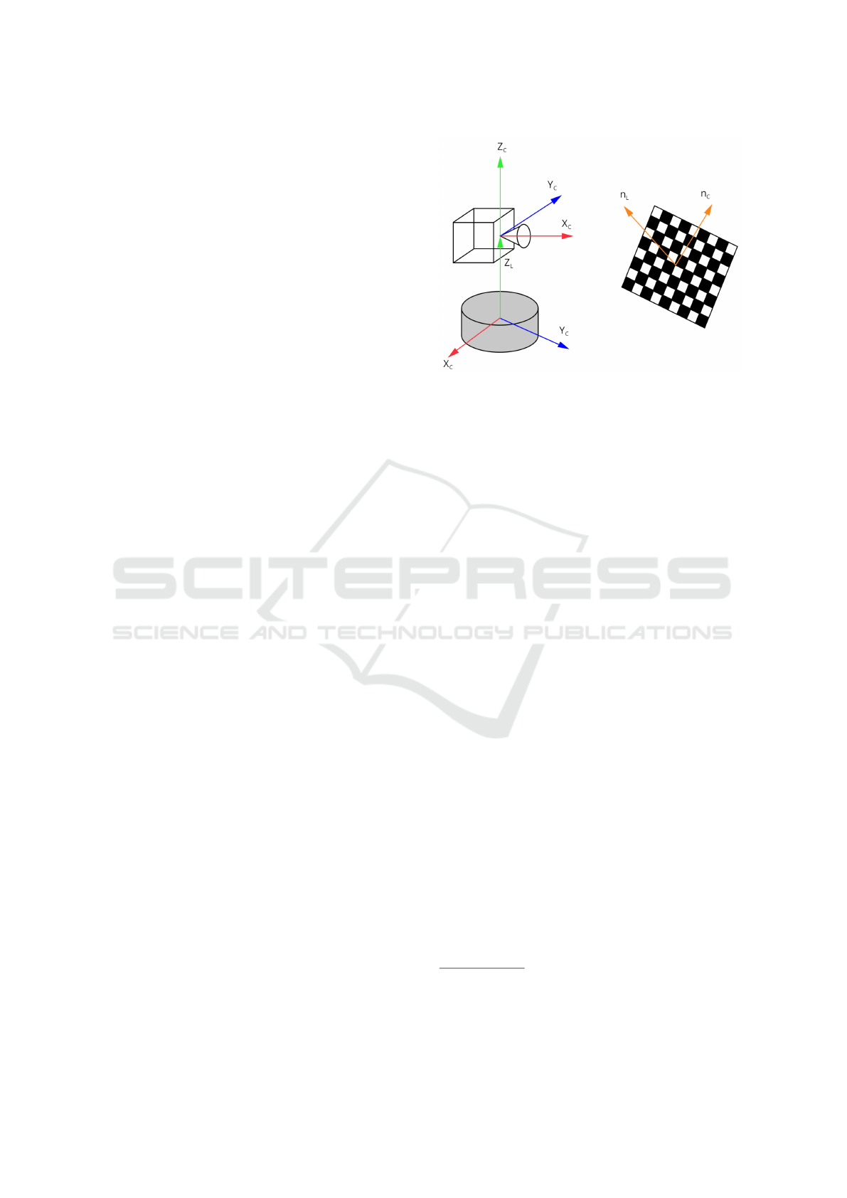
Figure 2: Schematic figure of Camera-LiDAR setup. Coor-
dinate sytems are highlighted by red, green and blue colors.
The main goal is to estimate the rotation around axis Z
C
.
K =


f k
u
0 u
0
0 f k
v
v
0
0 0 1


. (1)
Finally, selecting the world coordinate system as the
own coordinate system of the LiDAR, we get the re-
lationship between the points of LiDAR point cloud
and pixels of the image. The pixel coordinates of the
original 3D point are


u
v
1


∼ K · R(p
L
− t). (2)
2.1 Restrictions
The method considers the pinhole camera model and
known intrinsic camera parameters.
The novelty of the proposed method comes from
our own 3D printed mount which connects the camera
on the top of the LiDAR. This connection allows us to
make several restrictions about the systems which in
turn will reduce the complexity of the extrinsic cali-
bration problem to approximating a single rotation (1-
DoF problem). The mounted LiDAR-camera system
can be seen in Figure 5.
The first restriction is the coincidence of the ver-
tical axes of the LiDAR and camera coordinate sys-
tems. This means, that given the basis vectors of the
LiDAR coordinate systems X
L
, Y
L
, and Z
L
; the ba-
sis vectors of the camera coordinate system X
C
, Y
C
,
and Z
C
, assuming that Z
L
and Z
C
are the coinciding
vertical axes
1
: the planes spanned by X
L
, Y
L
and X
C
,
1
An important observation is that usually in the camera
coordinate system the Z axis points forward, the Y axis is
the vertical pointing down and the X axis points to the right.
In our case, the camera coordinate system is as in Figure 2.
LiDAR-camera Calibration in an Uniaxial 1-DoF Sensor System
731

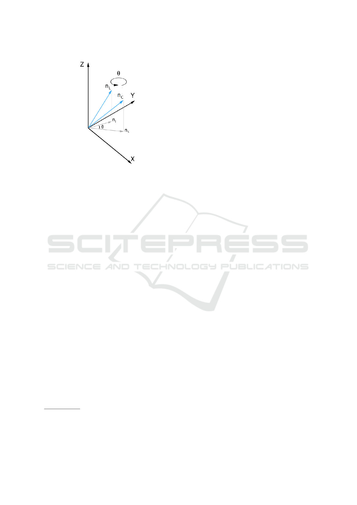
Figure 3: The goal of our calibration method is to estimate
the rotation angle θ around axis Z.
Y
C
respectively are parallel to each other illustrated
in Figure 2. This yields to the equality of the rota-
tions around the X and Y to the identity transforma-
tion R
X
= R
Y
= I. The free parameter of the rota-
tion came only from the rotation around the vertical Z
axis:
R = R
Z
(θ) =


cosθ −sinθ 0
sinθ cos θ 0
0 0 1


. (3)
Our second restriction is, that the translation vector
t =

0 0 t
Z

T
is known from the schematics of the
devices and the 3D printed mount.
The problem can be reduced to calculate a single
rotation around the vertical axis, i.e., angle θ if the
camera matrix K and the one translation parameter
t
z
are known. Given these restrictions, Equation (2)
modifies as follows


u
v
1


∼ K · R
Z
(θ) ·


p
x
p
y
p
z
−t
z


. (4)
2.2 Uniaxial Calibration
The target of the proposed extrinsic calibration
method is a plane with a checkerboard pattern printed
on it. This plane can be detected relatively easily on
both the image and in the LiDAR point cloud.
After the plane detection, we calculate the nor-
mal vector of the checkerboard in both the LiDAR
and camera coordinate system, these normal vectors
The proper alignment and rotation of the coordinate sys-
tems is an implementation problem that highly depends on
the available sensors, but is easily solvable by 90
◦
degree
rotations.
are denoted as n
L
and n
C
respectively. The follow-
ing equation holds between the two normal vectors:
n
L
= R
Z
·n
C
, which uses the same rotation as in Equa-
tion (3) visualized in Figure 3.
2.2.1 Plane Normal from the Point Cloud
At first, the plane points are selected manually. The
output is a subset of the point cloud containing as
few outliers as possible. This step is executed non-
automatically, because the plane of the checkerboard
is not necessarily the most prominent plane in the
whole scene of the point cloud. After the point classi-
fication, the LO-RANSAC (Lebeda et al., 2012) algo-
rithm can estimate the plane and its normal vector in
the LiDAR coordinate system based on the candidate
plane points.
2.2.2 Plane Normal from Image
In order to get the normal vector of checkerboard
plane in the camera coordinate system, not all of the
plane parameters are needed: a homography decom-
position can determine the required normal vector.
The input of the homography estimation are two
corresponding coplanar point sets. The first set of
points are the detected checkerboard corners in the
image of the camera. The second set of points will
be in the form of (0, 0), (0, 1), ..., (1, 0), (1, 1), ..., (n−
1, m − 1) (given a checkerboard pattern with size
n × m and with unit length squares), derived from a
virtual camera with an intrinsic matrix of K = I.
The homography matrix is defined by the n × m
coplanar point pairs. The homography is estimated
by the standard Direct Linear Transformation (DLT)
technique (Hartley and Zisserman, 2003). This ho-
mography is decomposed as written in (Malis and
Vargas, 2007), and the normal vector of the checker-
board in the camera coordinate system is obtained.
2.2.3 Rotation Form Normal Vectors
We determined the normal vector of the checkerboard
in both the LiDAR and the camera coordinate sys-
tems: n
L
=

x y z

T
and n
C
=

x
0
y
0
z
0

T
. Be-
cause of our assumption that the horizontal planes of
LiDAR and camera coordinate systems are parallel,
the depth coordinate becomes z = z
0
. If the projec-
tion of the normal vectors to the horizontal plane are
n
l
=

x y

T
and n
c
=

x
0
y
0

T
(see in Figure 3),
the equation of the rotation between the two vectors
yields to
R(θ) · n
l
=

cosθ − sinθ
sinθ cos θ

·

x
y

=

x
0
y
0

= n
c
. (5)
VISAPP 2022 - 17th International Conference on Computer Vision Theory and Applications
732

After rearranging the equation:

x −y
y x

·

cosθ
sinθ

=

x
0
y
0

. (6)
Let use the substitutions as follows
F =

x −y
y x

, g =

cosθ
sinθ

, h =

x
0
y
0

. (7)
The unknown calibration parameter can be de-
fined as the solution of the minimization problem
argmin
g
kFg − hk
2
subject to kgk
2
= 1. An algo-
rithm for computing the optimal result for this type of
problems is given in the appendix. The optimal angle
is obtained via calculating the roots of a four-degree
polynomial.
One pair of images is sufficient to perform the cal-
ibration. Notwithstanding, an overdetermind scenario
with more corresponding point cloud-image pairs can
increase the precise approximation of the rotation.
Assuming k number of image pairs, k normal vector
pairs can be gathered after the LO-RANSAC process
and the homography decomposition:
n
l,1
=

x
1
y
1

T
, . . . , n
l,k
=

x
k
y
k

T
,
n
c,1
=

x
0
1
y
0
1

T
, . . . , n
c,k
=

x
0
k
y
0
k

T
.
If k image pairs are considered, Equation 6 can be
written as follows:






x
1
−y
1
y
1
x
1
.
.
.
.
.
.
x
k
−y
k
y
k
x
k






·

cosθ
sinθ

=






x
0
1
y
0
1
.
.
.
x
0
k
y
0
k






. (8)
Finally, the method discussed in the appendix en-
sures the optimal solution for the only unknown cali-
bration parameter θ.
3 EXPERIMENTAL RESULTS
Qualitative and quantitative testing of the proposed
method was carried out on both real and virtually gen-
erated images and point clouds compared to a concur-
rent calibration process in MATLAB. In this section,
we analyze the results and evaluate the precision of
the tested approaches.
3.1 Real Data
We gathered point cloud-image pairs using a Vel-
doyne VLP-16 LiDAR and a Hikvision MV-CA020-
20GC sensor with high-quality Fujinon SV-0614H
Table 1: Standard deviation of the calculated rotations on
the different data sets measured in degrees. One by one:
only a single image used for calibration; One by one*: one
image used, but outliers are filtered out; 10 imgs.: overde-
termined estimation run for 10 randomly selected images.
The best result is highlighted in every test case.
Data set One-by-one One-by-one* 10 imgs.
#1 12.1753 2.3022 0.9759
#2 27.2212 2.3786 1.0583
#3 38.5715 0.6895 1.0392
#4 0.9453 - 0.4899
#5 28.9916 1.2363 4.0653
lenses. The non-perspective distortion of the lenses
is negligible. The camera was mounted on top of the
LiDAR with our special 3D printed mount. The data
were collected in different settings and with different
chessboards. Five data sets were gathered in different
places: in an office, in a garage, and in a parking lot
with three different chessboards. The sizes are from
4 × 5 to 9 × 10. Some input images can be seen in
Figure 4.
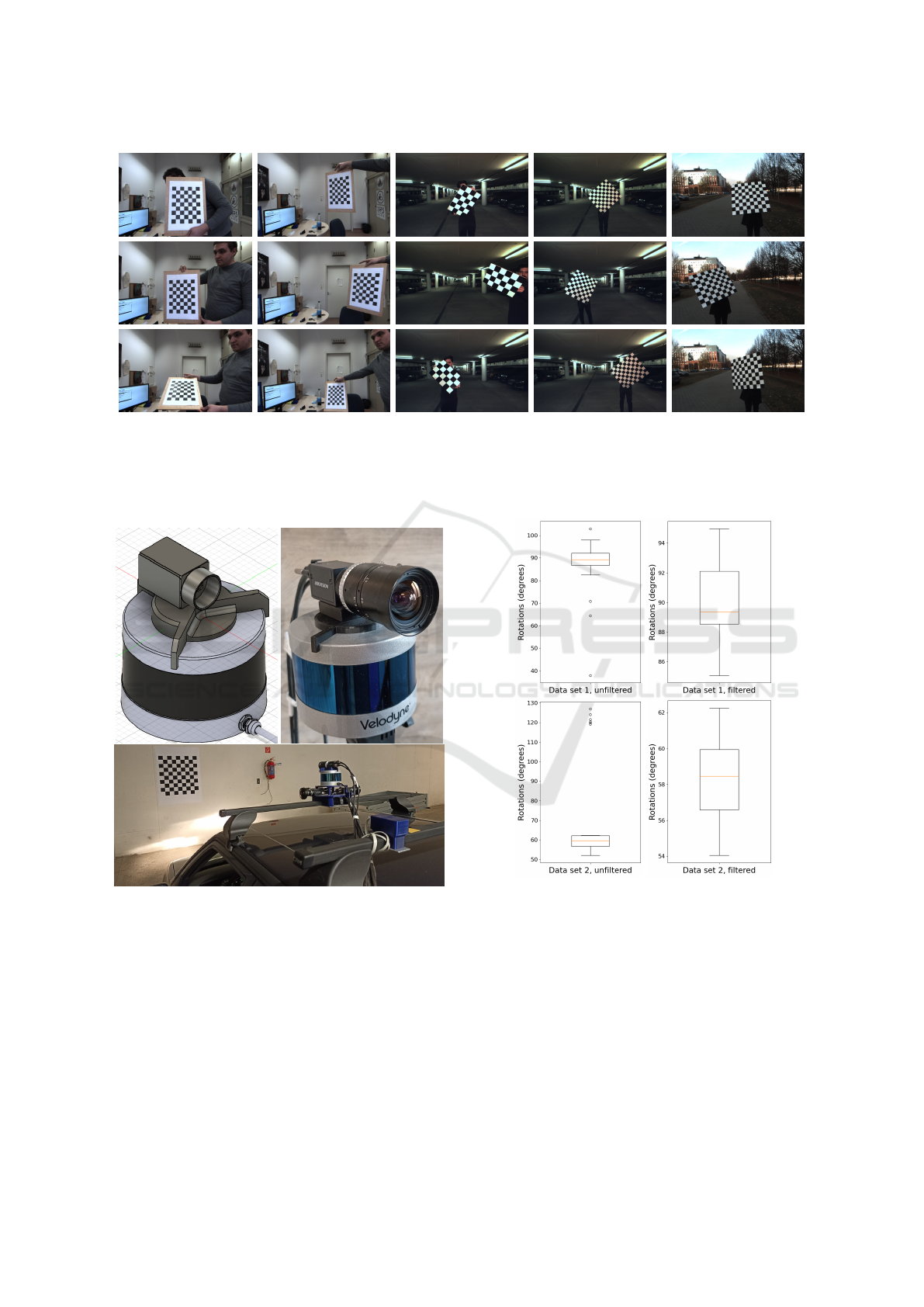
3.1.1 Precision of Estimated Rotation Angle
The first experiment examines the precision of angle
estimation. On every data set, the calibration was per-
formed one by one on each image – point cloud pair.
Our quantitative evaluations are based on the stan-
dard deviation of the estimated angles. The results
are listed in Table 1, where we concentrated on deter-
mining the precision of the results. Best results are
highlighted by bold numbers in every scenario. The
data were filtered from the outliers (illustrated in the
boxplots as separated dots). To evaluate the precision,
first, the angles are obtained one by one from LiDAR-
camera pairs. Thus, the proposed method is called for
the minimal case. Then ten chessboard planes are ran-
domly selected, and the over-determined algorithm is
performed. The best results are around 1
◦
on average.
The boxplots of the angles are pictured in Fig-
ures 6 and 7. Remark, that there are no outliers for
data set 4. The calculated rotation angles have a big
standard deviation because of outliers in the data set.
The outliers are filtered by boxplot, and the deviations
are recalculated. We also performed the calibration
on ten image-point cloud pairs at a time. From the fil-
tered data set, 10 randomly selected pairs were taken
multiple times, and a rotation angle was determined
with them.
Based on this test, it is obvious that outlier filtering
is important to obtain more precise results. We can
also note that in most cases using 10 images to per-
form the calibration produces more accurate results.
LiDAR-camera Calibration in an Uniaxial 1-DoF Sensor System
733

Data set 1 Data set 2 Data set 3 Data set 4 Data set 5
Figure 4: Some input image examples of the five different real data sets. The images and point clouds in data set 1 and 2
were taken in an office with a small 7x9 chessboard with 31mm square size. Data set 3 was gathered in a garage with a 60mm
square sized 4x6 chessboard. With data set 4 and 5 we were using a large 81mm square sized 9x10 chessboard in a garage
and in an outside parking lot.
Figure 5: Camera-LiDAR setup. A special, 3D printed fix-
ation used to connect the devices. Top left: 3D model of
equipment. Top rigth: Realized Camera-LiDAR pair. Bot-
tom: Proposed equipment mounted on the top of a car. A
single chessboard is used for calibration.
The resulting deviation values suggest that the
need for re-calibration can be detected if the fixation
error is larger than 1
◦
–2
◦
.
3.1.2 Point Cloud Colorization
We present the results of our extrinsic calibration
method by point cloud colorization and projecting
Figure 6: Boxplot of the rotations calibrated separately on
each image pair before and after filtering, on data sets 1 and
2.
the points of the point cloud back to the image. Li-
DAR point clouds do not contain color information
even if there is an intensity value for each point, how-
ever, they represent the reflectivity of the illuminated
points. RGB color data can be retrieved from camera
pixels if the LiDAR and camera are calibrated to each
other. In these experiments, this calibration is carried
out by the proposed method.
Figure 8 shows the examples when the LiDAR
points are projected to the images. The chessboard-
VISAPP 2022 - 17th International Conference on Computer Vision Theory and Applications
734

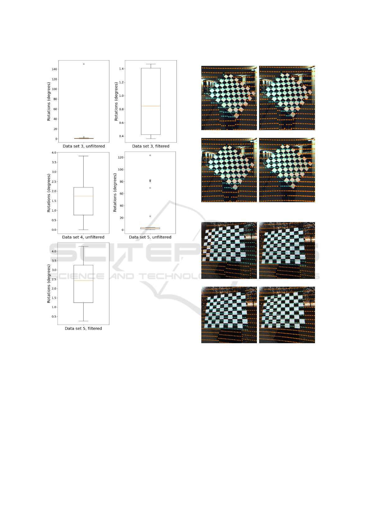
Figure 7: Boxplot of the rotations calibrated separately on
each image pair before and after filtering, on data sets 3, 4
and 5. Note: on data set 4, no outliers were found.
related points are colored by blue in the images. The
accuracy of the results can be visually checked at the
border of the chessboards. Colorized point clouds can
also be seen in Figure 9.
We compared our results with the LiDAR-camera
calibration toolbox (Zhou et al., 2018) of MATLAB.
It is important to note, that this toolbox couldn’t per-
form a calibration on several data sets, because of the
low resolution of the LiDAR available. Our method
does not have such problems.
Another important case is when the chessboard is
on the wall as in Figure 5. This mounting does not
Data set 4
Proposed – all imgs. Proposed – 10 imgs.
Proposed – 1 img. MATLAB
Data set 5
Proposed – all imgs. Proposed – 10 imgs.
Proposed – 1 img. MATLAB
Figure 8: These images are from data set 4 and 5. After
the calibration, the 3D points were projected back onto the
image. The points corresponding to the chessboard plane
can be seen in blue, all of the other back-projected LiDAR
points are orange.
affect our algorithm, because the only information we
need is the normal vector of the plane of the chess-
board in contrast to the MATLAB calibration method
which is highly dependent on the size and orienta-
tion of the chessboard. The plane of the large wall
can be detected by the well-known RANSAC (Fis-
chler and Bolles, 1981) algorithm. In the future, the
re-calibration and automatic detection of the chess-
LiDAR-camera Calibration in an Uniaxial 1-DoF Sensor System
735

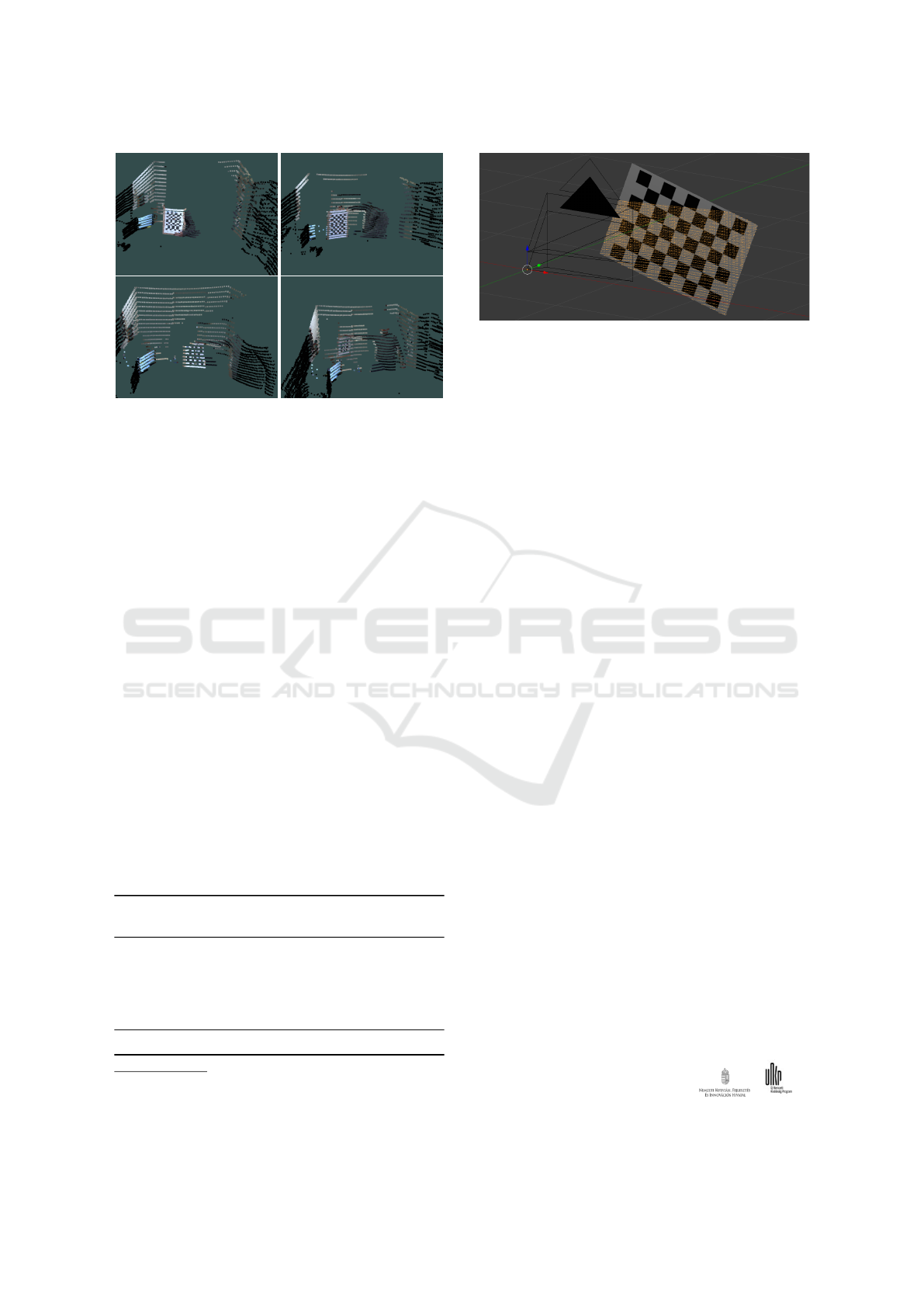
Figure 9: Colored point clouds on data sets 1 and 2 using
the calibration results of the proposed method.
boards plane in the LiDAR point cloud can be solved
this way, by assuming that the chessboard is mounted
on the wall. The largest plane in front of the car will
be that wall and detection of the chessboard can be
enhanced by also using the intensity information of
the scan.
3.2 Virtual Data
Multiple image and point cloud pairs were generated
at different angles using Blensor
2
. The setup of the
virtual camera and LiDAR can be seen in Figure 10.
At each known rotation angle, we can evaluate the ob-
tained rotation angle as the ground truth (GT) values
are known from the simulator.
The results are seen in Table 2. Results for five
different setups are compared, the ground truth angles
are from 0
◦
to 180
◦
. The average error of the approxi-
mated rotation with the proposed extrinsic calibration
method is only 0.1009°. It suggests that high-quality
angle estimation is possible using the proposed cali-
bration method.
Table 2: Calibration error of the proposed method on virtu-
ally generated data.
Rotation angle
Error
Ground truth Estimated
0° 0.0000° 0.0000°
45° 44.9032° 0.0976°
90° 89.6333° 0.3660°
135° 134.9589° 0.0410°
180° 179.9999° 2.05°×10
−7
Average error 0.1009°
2
Blensor is an open source simulation package for LI-
DAR and Kinect sensors that cooperates with the computer
vision tool Blender. See www.blensor.org for the details.
Figure 10: Setup of virtual LiDAR and camera in Blensor
with chessboard and captured LiDAR point cloud.
4 CONCLUSION
In this paper, we proposed a novel camera-LiDAR
calibration method, overviewed the restrictions of the
test environment, and the main steps of our frame-
work. In our setup, the camera is mounted on top
of the LiDAR using a special 3D-printed fixation,
and the DoF for calibration is reduced to one. We
showed how this problem can be optimally solved in
the least-squares sense. Both the minimal and the
over-determined cases were discussed. For the mini-
mal case, only one planar checkerboard pattern is re-
quired. We examined that the proposed method can
be applied to recalibrate a camera-LiDAR setup if the
fixation is changed during the vibration of the moving
vehicles on which the devices are mounted. During
synthetic and real-world tests, the proposed method
had an error of around 1°.
ACKNOWLEDGEMENTS
Our work is supported by the project EFOP-3.6.3-
VEKOP-16-2017- 00001: Talent Management in Au-
tonomous Vehicle Control Technologies, by the Hun-
garian Government and co-financed by the Euro-
pean Social Fund. L. Hajder also thanks the sup-
port of the ”Application Domain Specific Highly
Reliable IT Solutions” project that has been im-
plemented with the support provided from the Na-
tional Research, Development and Innovation Fund
of Hungary, financed under the Thematic Excellence
Programme TKP2020-NKA-06 (National Challenges
Subprogramme) funding scheme. T. T
´
ofalvi has been
supported by the
´
UNKP-21-1 New National Excel-
lence Program of the Ministry for Innovation and
Technology from the source of the National Research,
Development and Innovation fund.
VISAPP 2022 - 17th International Conference on Computer Vision Theory and Applications
736

REFERENCES
Alismail, H. S., Baker, L. D., and Browning, B. (2012). Au-
tomatic calibration of a range sensor and camera sys-
tem. In 2012 Second Joint 3DIM/3DPVT Conference:
3D Imaging, Modeling, Processing, Visualization &
Transmission (3DIMPVT 2012), Pittsburgh, PA. IEEE
Computer Society.
Fischler, M. and Bolles, R. (1981). RANdom SAmpling
Consensus: a paradigm for model fitting with appli-
cation to image analysis and automated cartography.
Commun. Assoc. Comp. Mach., 24:358–367.
Frohlich, R., Kato, Z., Tr
´
emeau, A., Tamas, L., Shabo,
S., and Waksman, Y. (2016). Region based fusion
of 3d and 2d visual data for cultural heritage objects.
In 23rd International Conference on Pattern Recog-
nition, ICPR 2016, Canc
´
un, Mexico, December 4-8,
2016, pages 2404–2409.
Geiger, A., Moosmann, F., Car, O., and Schuster, B. (2012).
Automatic camera and range sensor calibration us-
ing a single shot. In IEEE International Conference
on Robotics and Automation, ICRA 2012, 14-18 May,
2012, St. Paul, Minnesota, USA, pages 3936–3943.
Gong, X., Lin, Y., and Liu, J. (2013). 3d lidar-camera ex-
trinsic calibration using an arbitrary trihedron. Sen-
sors, 13(2).
Hartley, R. I. and Zisserman, A. (2003). Multiple View Ge-
ometry in Computer Vision. Cambridge University
Press.
Lebeda, K., Matas, J., and Chum, O. (2012). Fixing the lo-
cally optimized RANSAC. In British Machine Vision
Conference, BMVC 2012, Surrey, UK, September 3-7,
2012, pages 1–11.
Malis, E. and Vargas, M. (2007). Deeper understanding of
the homography decomposition for vision-based con-
trol. Research report.
Pandey, G., McBride, J., Savarese, S., and Eustice, R.
(2010). Extrinsic calibration of a 3d laser scanner and
an omnidirectional camera. In 7th IFAC Symposium
on Intelligent Autonomous Vehicles, volume 7, Leece,
Italy.
Pandey, G., McBride, J. R., Savarese, S., and Eustice, R. M.
(2012). Automatic targetless extrinsic calibration of a
3d lidar and camera by maximizing mutual informa-
tion. In Proceedings of the AAAI National Conference
on Artificial Intelligence, pages 2053–2059, Toronto,
Canada.
Park, Y., Yun, S., Won, C. S., Cho, K., Um, K., and Sim, S.
(2014). Calibration between color camera and 3d lidar
instruments with a polygonal planar board. Sensors,
14(3):5333–5353.
Pusztai, Z., Eichhardt, I., and Hajder, L. (2018). Accurate
calibration of multi-lidar-multi-camera systems. Sen-
sors, 18(7):2139.
Rodriguez F, S., Fremont, V., and Bonnifait, P. Extrinsic
calibration between a multi-layer lidar and a camera.
T
´
oth, T., Pusztai, Z., and Hajder, L. (2020). Automatic
lidar-camera calibration of extrinsic parameters using
a spherical target. In 2020 IEEE International Con-
ference on Robotics and Automation (ICRA), pages
8580–8586.
Ve
´
las, M.,
ˇ
Span
ˇ
el, M., Materna, Z., and Herout, A.
(2014). Calibration of rgb camera with velodyne lidar.
In WSCG 2014 Communication Papers Proceedings,
volume 2014, pages 135–144. Union Agency.
Zhang, Q. and Pless, R. (2004). Extrinsic calibration of a
camera and laser range finder (improves camera cali-
bration). In 2004 IEEE/RSJ International Conference
on Intelligent Robots and Systems, Sendai, Japan,
September 28 - October 2, 2004, pages 2301–2306.
Zhang, Z. (2000). A flexible new technique for camera cal-
ibration. IEEE Transactions on Pattern Analysis and
Machine Intelligence, 22(11):1330–1334.
Zhou, L., Li, Z., and Kaess, M. (2018). Automatic extrinsic
calibration of a camera and a 3d lidar using line and
plane correspondences. In 2018 IEEE/RSJ Interna-
tional Conference on Intelligent Robots and Systems,
IROS 2018, Madrid, Spain, October 1-5, 2018, pages
5562–5569.
APPENDIX
Solution of argmin
Y
k
FG − H
k
2
Subject to
k
g
k
2
= 1.
The objective is to show how the equation Fg = h can
be optimally solved, in the least squares sense, sub-
ject to g
T
g = 1. Cost function J can be written using
Lagrangian multiplier λ as follows:
J = (Fg − h)
T
(Fg − h) + λg
T
g.
The optimal solution is given by the derivative of J
w.r.t. vector g as
∂J
∂g
= 2F
T
(Fg − h) + 2λg = 0.
Therefore the optimal solution is g =

F
T
F + λI

−1
F
T
h. For the sake of simplicity,
let us denote vector F
T
h by r and the symmetric
matrix F
T
F by L. Then g = (L + λI)
−1
r. Finally,
constraint g
T
g = 1 has to be considered as
r
T
(L + λI)
−T
(L + λI)
−1
r = 1. (9)
The inverse matrix can be written as
(L + λI)
−1
=
adj(L +λI)
det(L +λI)
,
where adj(L + λI) and det(L +λI) denote the adjoint
matrix
3
and the determinant of matrix L +λI, respec-
tively. This can be substituted into Eq. 9 as follows:
r
T
adj
T
(L + λI)adj(L + λI) r = det
2
(L + λI).
3
Adjoint matrix is also called as the matrix of cofactors.
LiDAR-camera Calibration in an Uniaxial 1-DoF Sensor System
737

Both sides of the equation contain polynomials. The
degrees of the left and right sides are 2n − 2 and 2n,
respectively. If the expression in the sides are sub-
tracted by each other, a polynomial of degree 2n is
obtained. Note that n = 2 in the discussed case, when
the single angle of a rotation is estimated. The opti-
mal solution is obtained as the real roots of this poly-
nomial. The vector corresponding to the estimated λ
i
,i ∈ {1, 2}, is calculated as g
i
= (L + λ
i
I)
−1
r. Then
the vector with minimal norm
k
Fg
i
− h
k
is selected as
the optimal solution for the problem.
VISAPP 2022 - 17th International Conference on Computer Vision Theory and Applications
738