Efﬁcient k-mer Indexing with Application to Mapping-free SNP

Genotyping

Mattia Marcolin, Francesco Andreace and Matteo Comin

Department of Information Engineering, University of Padua, Via Gradenigo 6/a, 35100 Padua, Italy

Keywords:

Genotyping, Mapping-free, k-mers Set Representation.

Abstract:

Advances in sequencing technologies and computational methods have enabled rapid and accurate identiﬁca-

tion of genetic variants. Accurate genotype calls and allele frequency estimations are crucial for population

genomics analyses. One of the most demanding step in the genotyping pipeline is mapping reads to the human

reference genome. Recently mapping-free methods, like Lava and VarGeno, have been proposed for the geno-

typing problem. They are reported to perform 30 times faster than a standard alignment-based genotyping

pipeline while achieving comparable accuracy. Moreover, these methods are able to include known genomic

variants in the reference making read mapping, and genotyping variant-aware. However, in order to run they

require a large k-mers database, of about 60GB, to be loaded in memory. In this paper we study the prob-

lem of genotyping using new efﬁcient data structures based on k-mers set compression, and we present a fast

mapping-free genotyping tool, named GenoLight. GenoLight reports accuracy results similar to the standard

pipeline, but it is up to 8 times faster. Also, GenoLight uses between 5 to 10 times less memory than the other

mapping-free tools, and it can be run on a laptop. Availability: https://github.com/CominLab/GenoLight.

1 INTRODUCTION

The discovery and characterization of sequence varia-

tions in human populations is crucial in genetic stud-

ies. A prime challenge is to efﬁciently analyze the

variations of a freshly sequenced individual with re-

spect to a reference genome and the available ge-

nomic variation data. Single nucleotide polymor-

phism (SNP) genotyping has been widely used in hu-

man disease-related research such as genome-wide

association studies (Stranger et al., 2011) and a recent

study on rare-disease diagnosis (NEJ, 2021).

The approaches to SNP genotyping can be

roughly divided into three categories: microarray

methods, sequencing alignment-based methods, and

alignment-free methods. The ﬁrst approach uses SNP

arrays (Pastinen and et al., 2000). SNP arrays are fast

and inexpensive; however, they can only hold a lim-

ited number of probes: the state-of-the-art Affymetrix

genome-wide SNP array 6.0 has only 906 000 SNP

probes, compared to 31 million known common SNPs

in dbSNP (build 150).

The second approach is based on high-throughput

whole-genome sequencing and read alignment. In

most NGS-based genotyping pipelines, the ﬁrst step

after sequencing a genome is to map each read to

the reference (Li and Durbin, 2010; Langmead and

Salzberg, 2012). Standard tools for genotyping (e.g.

Samtools mpileup (Li et al., 2009) and GATK Hap-

lotypeCaller (McKenna and et al., 2010)) require

this mapping information for every read before being

able to call variants. Yet, despite recent advances in

speed (Marco-Sola et al., 2012; Siragusa et al., 2013;

Yorukoglu et al., 2016; Zaharia et al., 2011), map-

ping still remains a computationally expensive step.

Furthermore, genotyping pipelines also include vari-

ant calling steps, signiﬁcantly increasing the total run-

time.

The third approach is based on high-throughput

whole genome sequencing followed by an alignment-

free sequence comparison (Zielezinski et al., 2017).

Alignment-free methods have been used to save com-

pute time and memory by avoiding the cost of full-

scale alignment (Vinga, 2014). The reliance on a

single reference human genome could introduce sub-

stantial biases in downstream analyses (Brandt et al.,

2015; G

unther and Nettelblad, 2019; Salavati et al.,

2019). Furthermore, including known variants in

the reference makes read mapping, variant calling,

and genotyping variant-aware. Alignment-free ap-

proaches have been applied to SNP genotyping (Sha-

jii et al., 2016; Sun and Medvedev, 2019). They

Marcolin, M., Andreace, F. and Comin, M.

Efﬁcient k-mer Indexing with Application to Mapping-free SNP Genotyping.

DOI: 10.5220/0010985700003123

In Proceedings of the 15th International Joint Conference on Biomedical Engineering Systems and Technologies (BIOSTEC 2022) - Volume 3: BIOINFORMATICS, pages 62-70

ISBN: 978-989-758-552-4; ISSN: 2184-4305

introduced two SNP genotyping tools named LAVA

and VarGeno, respectively, which build an index from

known SNPs (e.g., dbSNP) and then use approxi-

mate k-mer matching to genotype the donor from se-

quencing data. LAVA and VarGeno have been re-

ported to perform 4 to 30 times faster than a standard

alignment-based genotyping pipeline while achieving

comparable accuracy. Recently, another alignment-

free genotyping tool, called MALVA (Denti et al.,

2019), has been able to handle indels. Remark-

ably, alignment-free methods provide in some cases

even better results than the most widely adopted

SNPs discovery pipeline (Shajii et al., 2016; Sun

and Medvedev, 2019). In addition, these tools pro-

vide a faster alternative to read mapping, and with

the increasing of sequencing capabilities, they are a

promising direction of investigation. However, they

require a large amount of memory for indexing k-

mers, about 60GB, and all tools can be run only on

a large server with adequate RAM. In this work, we

introduce GenoLight that will address this problem

with new efﬁcient data structures based on k-mer set

compression.

2 PRELIMINARIES

In this section, we report the basic concepts about the

functionality of VarGeno (Sun and Medvedev, 2019)

and the notation used inside this document to explain

GenoLight more clearly. We describe VarGeno be-

cause it is the fastest tool and also because the other

methods follow a similar paradigm. Given a database

of biallelic SNPs l

encoded as VCF (Variant Call-

ing Format) ﬁle, a database of reads from the genome

that we want to genotype, and a reference genome

, VarGeno produces a VCF ﬁle containing the most

probable genotype for each variant inside l

. SNPs

not contained in l

are not genotyped.

The VarGeno pipeline consists of two phases.

During the ﬁrst phase, VarGeno maps each read r in-

side the database on G

, in an alignment-free fashion,

and then in the genotyping phase it uses the align-

ment information to detect the SNPs. To understand

how the mapping is performed, we need to introduce

some deﬁnitions and concepts. We denote by G

the

genome obtained by G

replacing, at each locus con-

taining an SNP ∈ l

, the alternative variant.

Conceptually, in this phase VarGeno extracts all

non-overlapping k-mer, with k= 32, from a read r and

searches for them in G

and G

. The position sup-

ported by a k-mer is the difference between the po-

sition in which the k-mer occurs inside the genome

and/or G

) and the position in which it appears

inside the read. The position supported by the largest

number of k-mers and that respect two constraints that

we will deﬁne later in this section is called the target

position (t

) and represents the initial position where

the read is mapped to G

or G

. We report a simple

example in Figure 1, in which the read r is split into

three non-overlapping k-mers, that are searched into

the two genomes. All three k-mers are in agreement

and support the target position 10.

To search k-mers in G

and G

efﬁciently,

VarGeno builds two dictionaries D

re f

and D

snp

using

Bloom ﬁlers. D

re f

stores the binary encoding of each

overlapping k-mer, with k = 32, from G

and the rel-

ative initials positions. K-mers that occur inside G

with a frequency greater than 10 are discarded be-

cause they likely lead to an incorrect calculation of

The same process could be used to build D

snp

from G

. However, the only k-mers not present in

re f

would be the 32 consecutive k-mers for each

SNP ∈ l

that contain the alternative variant. So,

VarGeno stores only such k-mers inside D

snp

in a bi-

nary encoding with the relative initials positions.

Using a speciﬁc search algorithm that involves the

use of D

re f

and D

snp

, VarGeno is able to efﬁciently

obtain all the initial positions of a k-mer in G

and

and thus establishes the target position of a read.

The presence of sequencing errors inside the reads

can lead to an incorrect calculation of t

. To solve

this problem, given a k-mer K, LAVA (Shajii et al.,

2016) calculates the initial position within G

re f

and

snp

not only by searching for K but also of all k-mers

belonging to his Hamming neighbourhood, denoted

by N(K). This set is composed of all k-mers having,

at most, a Hamming distance equal to 1 from K. We

observe that |N(k)| = 3k + 1. In this way, k-mers that

would be present in G

or in G

, but are affected by a

single sequencing error contribute to the correct cal-

culation of the target position. To reduce the search

space and thus increase the temporal performance,

VarGeno uses quality scores to choose which k-mer

∈ N(K) to search within D

re f

and D

snp

(besides ob-

viously K). In particular, it searches for the k-mers

∈ N(K) whose character K

[i], 0 ≤ i ≤ 31 that dif-

ferentiates them from K has a quality score value Q[i]

higher than a certain threshold. We can now deﬁne

the constraint that the k-mer that supports position t

must satisfy. Let t

be the position supported by the

largest number of k-mers, to be the target position,

these two conditions must hold:

1. At least one of the k-mers extracted from r sup-

ports t

;

2. Let K

and K

be two k-mers extracted from r, x 6=

y. At least one k-mer belonging to the set N(K

)

Efﬁcient k-mer Indexing with Application to Mapping-free SNP Genotyping

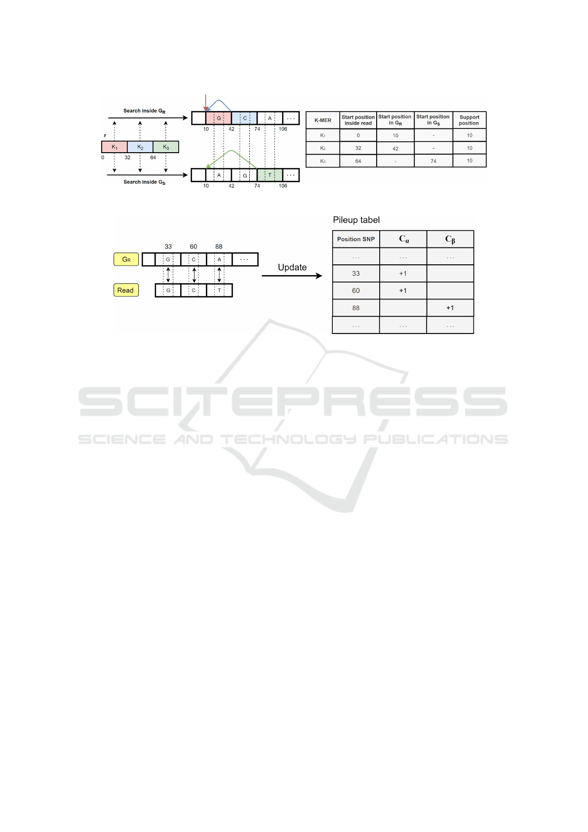
Figure 1: An example of target position calculation.

Figure 2: Pileup table update.

and one k-mer belonging to the set N(K

) must

support t

;

If more than one position has the same maxi-

mum number of supporter k-mers and respects these

two constraints, the current read is considered not

mapped. In general, if a read is not mapped, Vargeno

tries to map its reverse complement of r, performing

the same steps described.

The size of non-overlapping k-mers extracted

from reads, and consequently the size of k-mers inside

the dictionary, is ﬁxed to 32 for the following reasons.

For the human genome, 85% of 32-mer have unit fre-

quency: this is fundamental for how t

is calculated.

The second reason is that the binary representation of

the k-mer can be stored exactly in a 64-bit variable

without wasting space in a 64-bit architecture.

Once the target position has been identiﬁed,

VarGeno checks if there are SNPs ∈ l

in the range

[t p, t p + |r|] within l

, where |r| is the length of the

read. If so, it proceeds with updating a data structure

called pileup table. For each SNP, there are two coun-

ters C

and C

. The ﬁrst is increased by one unit if a

read contains the reference variant, and the second is

increased by one unit if the read contains the alterna-

tive variant. An example is shown in Figure 2.

Once all the dataset reads are processed, using the

data contained in the pileup table, VarGeno proceeds

with the genotyping phase, using the Bayesian statis-

tical framework (Sun and Medvedev, 2019).

3 METHODS

The basic idea of LAVA and VarGeno is to build two

dictionaries of k-mers, one with all k-mers from the

reference genome and another with the k-mers cov-

ering known SNPs. In LAVA, these dictionaries are

implemented with a hash table where all k-mers are

explicitly stored; instead, VarGeno uses a Bloom ﬁl-

ter. Both these data structures need to be loaded into

memory for efﬁcient queries, and they require about

60-63 GB of RAM. However, the size of these dic-

tionaries can be reduced because most of the infor-

mation carried by a k-mer is redundant. Given two

overlapping k-mers, it is possible to reassemble them

into a single (k+1)-mer, thus reducing the storage re-

quirement by k-1 bases. In GenoLight we further

exploit this observation: a set of k-mers, associated

with known SNPs, is assembled into a string, or set

of strings, that contains all of them. This proce-

dure allows us to store the whole dictionary in linear

form, reducing the memory requirements from O(kn)

to O(n) without losing information.

This problem is closely related to the represen-

tation and compression of k-mer sets, which has at-

tracted the attention of many researchers recently

rinda et al., 2021; Rahman and Medvedev, 2020).

K-mer sets are widely used in many bioinformatics

applications (Storato and Comin, 2021; Qian et al.,

2018; Marchiori and Comin, 2017; Qian and Comin,

2019; Andreace et al., 2021a; Andreace et al., 2021b).

BIOINFORMATICS 2022 - 13th International Conference on Bioinformatics Models, Methods and Algorithms

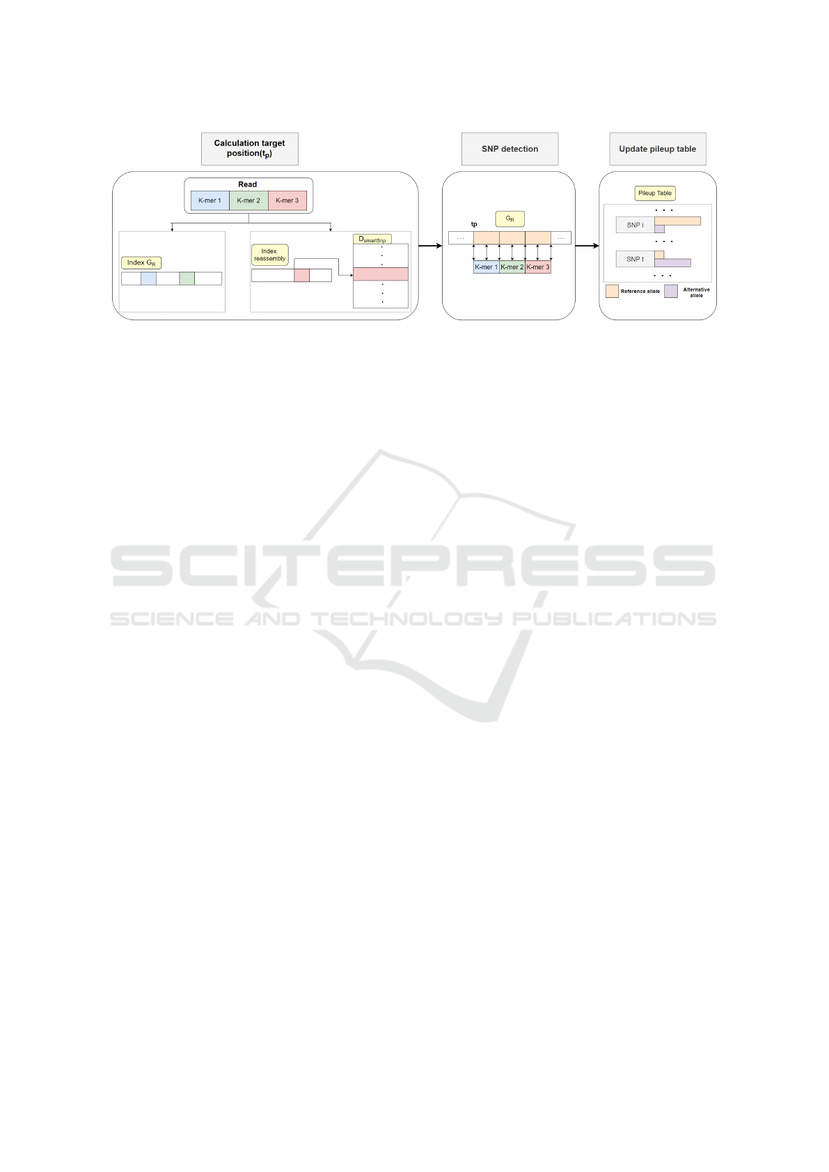
Figure 3: An overview of the genotyping pipeline of GenoLight.

In fact, a k-mers set can be represented by its De

Bruijn graph. Instead of explicitly storing the graph, it

can be compressed by assembling the graph and com-

puting a string that traverses all nodes in the graph

only once. However, this problem is far from triv-

ial, like traditional assembly, and the algorithms pro-

posed in (B

rinda et al., 2021; Rahman and Medvedev,

2020) will not produce a single string that traverses all

nodes. Instead, the results of this assembly are a set of

strings, called unitigs, that describe and cover the De

Bruijn graph. These techniques have been success-

fully applied to quality value compression (Shibuya

and Comin, 2019a; Shibuya and Comin, 2019b).

In this work, we use these memory efﬁcient data

structures to calculate the target position of a read.

The aim of this project is to develop a tool that can

be run on a personal computer without the need of a

server with a large amount of RAM. Moreover, we

implement an efﬁcient search algorithm with time

performance similar to that of other alignment-free

methods.

In order to use the efﬁcient representation of k-

mer set (B

rinda et al., 2021), the dictionary D

snp

needs to be replaced by two new data structures, the

RI reassembly index and a new dictionary named

SmartSnp

. Recall that D

snp

contains all k-mers ex-

tracted from G

that cover an SNP. The binary en-

coding of these 32-mer isn’t stored directly inside

SmartSnp

. Instead, these k-mers are compressed into

a string called the reassembly index, indicated with

RI, in which each k-mer extracted from G

is present

with unit frequency. In order to create the reassem-

bly index RI we use the Prophasm k-mer set assem-

bler (B

rinda et al., 2021). Given a dataset of k-mers,

Prophasm creates a string that contains all input k-

mers exactly once. However, this compressed repre-

sentation has two characteristics that we need to con-

sider. First, depending on the input k-mers set, it may

not be possible to assemble all of them into a single

string. Instead, Prophasm produces a set of strings

that assemble and cover all input k-mers. The sec-

ond issue is that a k-mer can be represented in the

reassembly index in the forward or reverse comple-

ment orientation. Unfortunately, the orientation can-

not be determined a priori. Moreover, if in the input

k-mer set two k-mers that are one the reverse com-

plement of the other, these two k-mers will be repre-

sented only once in the reassembly index and not as

two separated k-mers. In summary, a set of k-mers

can be compressed using Prophasm into a reassem-

bly index, with a substantial saving in terms of space.

However, some important information might be lost

during this process, and for this reason we introduce

a new dictionary named D

SmartSnp

In GenoLight, to compute the target position of

a k-mer and the associated SNP position, we need to

store for each k-mer in the reassembly index: the orig-

inal position in the reference; its direction, forward

or reverse; and the associated SNP. Instead of storing

the k-mers in binary format as in D

snp

, every k-mer

in RI can be identiﬁed by its position in the reassem-

bly index. The new dictionary D

SmartSnp

contains a

set of records, one for each position in the reassembly

index RI. In a record, the most important informa-

tion is the original position of the k-mer inside G

While the binary encoding of a 32-length k-mer re-

quires 64 bits to be stored, the integer representing

the k-mer’s position can be stored using 32 bits. This

reduces the size of D

SmartSnp

compared to D

snp

by 32

bits for each record. The second information in the

record is the SNP position with respect to the k-mer.

To correctly calculate the target position, it is essential

to keep track of the k-mer orientation inside RI with

respect to G

. This information is also stored in the

k-mer record inside D

SmartSnp

. If the k-mer appears

both as a forward and reverse complement in G

, then

in the reassembly index it will appear only once, in

one of the two directions. In this case, the information

on the k-mer that is present inside the RI is stored in

SmartSnp

, while the information on other k-mer will

Efﬁcient k-mer Indexing with Application to Mapping-free SNP Genotyping

be stored in a small auxiliary data structure.

The read mapping phase of GenoLight is simi-

lar to that of VarGeno. A read is split into non-

overlapping k-mers, and these k-mers are searched in

the reference sequence G

and the alternative refer-

ence G

, in order to detect a candidate target position,

see Figure 3. However, the representation of these

references is different with respect to VarGeno. In

VarGeno, both G

and G

are represented by Bloom

ﬁlters. Whereas in GenoLight, we use the original ref-

erence sequence for G

, and the reassembly index RI

and D

SmartSnp

for G

. Both G

and RI contain a set of

sequences in which we want to search for k-mers.

In order to allow for fast queries we use a vari-

ant of the FM-index (Ferragina and Manzini, 2000),

the FDM-Index also used in BWA (Li and Durbin,

2010). GenoLight uses FDM-Index to index G

and

RI, and the bound backtracking algorithm described

in (Li and Durbin, 2010) to search for k-mers in-

side it. This algorithm solves the inexact string match

problem and is used by the Burrows-Wheeler Aligner

(BWA). BWA performs local alignment of reads on a

genome according to the seed-and-extend alignment

paradigm. To perform the seeding phase efﬁciently, it

indexes the reference genome using FDM-Index and

performs searches with at most m mismatches to ﬁnd

areas with high similarity using this algorithm. We

adapt this library allowing only for one mismatch and

using the additional constraint provided by quality

values so that possibly wrong bases are not aligned.

A pseudocode of the read mapping phase is re-

ported above. Each read is decomposed into non-

overlapping k-mers. For each k-mer we compute its

neighbourhood also using the quality values. Then,

these k-mers are searched in the reference genome

through its index. If a match is found, these positions

are stored in the vector P. To obtain the position p

where a k-mer k occurs inside G

, the alternative ref-

erence, GenoLight ﬁrst identiﬁes the starting position

reassembly

of k inside RI. Next, it accesses D

SmartSnp

using p

reassembly

as key to get p

. To efﬁciently

search k in RI, RI is also indexed using FDM-Index.

Once all matching positions have been stored in the

vector P, we can compute the target position of the

read, as in Figure 1. Finally, we can update the pileup

table and compute the genotyping using the Bayesian

statistical framework as in (Sun and Medvedev, 2019;

Shajii et al., 2016).

4 RESULTS

In this section, we report the results obtained by the

tools GenoLight, VarGeno (Sun and Medvedev, 2019)

Algorithm 1: GenoLight search.

Input:

IndexG: FDM-Index of the reference genome G

IndexRI: FDM-Index of the reassembly RI

SmartSnp

: Dictionary containing k-mer having the

alternative allele

r : Read to map into the reference genome

Q[K] : Quality scores associated with a k-mer K

extracted from r

Output

: target position of reads

Start

S ← ExtractNonOverlapKmer(r)

P ←

for each K ∈ S do

N(K)

← Filter(N(K), Q[K])

P ← SearchRe f erenceGenome(N(K)

, IndexG)

for each k ∈ N (K)

reassembly

← SearchRI(k, IndexRI)

← D

SmartSnp

reassembly

]

P ← P

← CalculateTargetPosition(P)

End

and Lava (Shajii et al., 2016), as well as the standard

alignment-based genotyping pipeline (BWA (Li and

Durbin, 2010) as aligner, and BCFtools (Li, 2011)

as variant caller). The analysis focuses on two fun-

damental points, the computation time and memory

taken to complete the alignment and genotyping pro-

cess, and the accuracy of the results obtained by the

respective tools.

4.1 Experimental Setup

The datasets used in this study are two sets of real

reads from the same individual (NA12878) from the

1000 Genomes Project (Project, 2008): SRR622461

with a coverage of 6X (40 GB) and SRR622457 with

a coverage of 10X (65 GB). These datasets have

been widely used for benchmarking in other stud-

ies (Shibuya and Comin, 2019a; Shibuya and Comin,

2019b; Shajii et al., 2016; Sun and Medvedev, 2019;

Monsu and Comin, 2021). For validation, we used

an up-to-date high-quality genotype annotation gen-

erated by the Genome in a Bottle Consortium (Zook

et al., 2019). The GIAB gold standard contains

validated genotype information for NA12878, from

14 sequencing datasets with ﬁve sequencing tech-

nologies, seven read mappers, and three different

variant callers. The number of SNPs validated for

BIOINFORMATICS 2022 - 13th International Conference on Bioinformatics Models, Methods and Algorithms

Table 1: Resources and Datasets used for testing.

DATASET DESCRIPTION

hg19 Reference genome

dbSNP Biallelic SNPs dataset (Sherry et al., 2001)

Affymetrix Affymetrix Genome-Wide Human SNP Array

NA12878 Gold standard from GIAB (Zook et al., 2019)

SRR622461 (Low Coverage) Dataset of reads with coverage 6X

SRR622457 (High Coverage) Dataset of reads with coverage 10X

NA12878 in the gold standard is 3.7M. The reference

genome used is hg19, also described as Genome Ref-

erence Consortium Human Build 37 (GRCh37). For

the SNPs dataset, we choose dbSNP (Sherry et al.,

2001), which contains human single nucleotide vari-

ations, and more speciﬁcally 11M SNPs biallelic,

and Affymetrix Genome-Wide Human SNP Array 6.0

with about 1M SNPs. A summary of the datasets used

for the evaluation is reported in Table 1.

To measure the accuracy, we use RTG Tools and

the SNP list which are also genotyped in the GIAB

gold standard. All tests were performed on a 14 lame

blade cluster DELL PowerEdge M600 where each

lame is equipped with two Intel Xeon E5450 at 3.00

GHz, 16GB RAM and two 72GB hard disk in RAID-

1 (mirroring).

4.2 Computational Resources: Time

and Memory

In this section we test the requirement of computa-

tional resources for all tools. Table 2 reports a sum-

mary of the results obtained for the two read datasets,

with the two SNP databases, for all tools.

We consider the standard alignment-based geno-

typing pipeline as the reference to compare the three

mapping-free algorithms. As expected, the standard

pipeline is always more time consuming while re-

quiring only 4 GB of memory. On the low coverage

dataset the standard pipeline requires 1929 minutes

to align 179 millions reads, that is more than 1 day

of computation. On this dataset VarGeno is able to

genotype the reads in only 59 and 44 minutes, de-

pending on the SNP databases, remaining the fastest

tool, thanks to the Bloom ﬁlter, as expected (Sun and

Medvedev, 2019). GenoLight is the second fastest

tool, it can process the low coverage dataset in 406

and 295 minutes, using the two SNP databases, which

results in a speed-up of 4.75x and 6.5x with respect to

the standard pipeline. LAVA is the slowest of the three

mapping-free methods.

If we consider the high coverage dataset, that con-

tains 287 million reads, the standard pipeline requires

2560 minutes, again more than one day of compu-

tation on a server. The time performance of the

mapping-free tools is similar to that of the low cov-

erage dataset. VarGeno is the fastest tool with 80 and

55 minutes, GenoLight needs 503 and 296 minutes,

and Lava requires 723 and 435 minutes, on the two

SNP databases. On the high coverage datasets, the

speed-up of GenoLight with respect to the standard

pipeline is 5.1x and 8.6x, for the two SNP databases.

GenoLight is again the second fastest tool; however,

on the high coverage dataset the speed-up w.r.t. stan-

dard pipeline increases.

In terms of memory requirement, the standard

pipeline is the least expensive, with only 4 GB of

RAM needed. For the mapping-free tools, the mem-

ory is mainly dominated by the size of the k-mers

database and the corresponding data structures, and

it varies only slightly with the number of the input

reads. On the smallest SNP database, e.g. Affymetrix,

GenoLight requires only 6 GB of RAM, whereas Lava

requires 57.6 GB and VarGeno about 59 GB. On the

largest SNP database, e.g. dbSNP, GenoLight needs

12.5 GB of memory, whereas Lava requires 60 GB

and VarGeno 63 GB.

In summary, only GenoLight and the standard

pipeline can run on a laptop with 16 GB of RAM

because the memory requirements of both methods

are low. However, GenoLight is much faster than the

standard pipeline, up to 8.6x.

4.3 Genotyping Accuracy

In this section we test the genotyping accuracy of all

tools on both datasets. The VCF ﬁle produced by the

standard pipeline and all mapping-free tools are com-

pared with the gold standard (Zook et al., 2019). In

Table 3 are shown the results in terms of accuracy, in

line with other studies (Shajii et al., 2016; Sun and

Medvedev, 2019).

For the Low Coverage dataset, the standard

pipeline has an accuracy of 93%. VarGeno and Geno-

Light have similar performance, varying from 91% to

93.5%, depending on the SNP databases. Lava shows

a lower accuracy in some cases. The different per-

formance of Lava can be explained by the fact that

it does not use quality value information, unlike the

Efﬁcient k-mer Indexing with Application to Mapping-free SNP Genotyping

Table 2: Performance results of the genotyping for all tools on various datasets.

Dataset SNP db Algorithm Time (d:h:m) RAM (GB)

Low Coverage

None Standard Pipeline 1:08:09 4

dbSNP

VarGeno 59 63.2

Lava 8:26 61

GenoLight 6:46 12.5

Affymetrix

VarGeno 44 58.9

Lava 5:18 57.6

GenoLight 4:55 6

High Coverage

None Standard Pipeline 1:18:40 4

dbSNP

VarGeno 1:20 63.242

Lava 12:03 60

GenoLight 8:23 12.5

Affymetrix

VarGeno 55 59

Lava 7:15 57.6

GenoLight 4:56 6

Table 3: Performance results of the genotyping for all tools on various datasets.

Dataset SNP db Algorithm Accuracy

Low Coverage

None Standard Pipeline 0.930

dbSNP

VarGeno 0.911

Lava 0.819

GenoLight 0.912

Affymetrix

VarGeno 0.935

Lava 0.935

GenoLight 0.934

High Coverage

None Standard Pipeline 0.969

dbSNP

VarGeno 0.949

Lava 0.845

GenoLight 0.951

Affymetrix

VarGeno 0.977

Lava 0.974

GenoLight 0.976

other two mapping-free methods.

On the High Coverage dataset, thanks to the 10X

coverage, all tools reported higher accuracy values.

In this case, the standard pipeline has an accuracy

of 96.9%. Also, on this dataset the behaviour of all

mapping-free tools is similar to the previous case.

VarGeno and GenoLight have similar accuracies, in

line with the standard pipeline, whereas Lava is less

precise.

In summary, among the mapping-free tools,

VarGeno and Genolight achieve the best overall per-

formance in terms of accuracy, in line with the stan-

dard pipeline. GenoLight reports precision results

comparable to VarGeno, but it uses between 5 and 10

times less memory than the other two tools. The stan-

dard alignment-based pipeline is extremely slow, and

it requires more than a day of computation on a clus-

ter. GenoLight achieves almost the precision levels

and memory usage of the standard pipeline while be-

ing signiﬁcantly faster, thus resolving the high mem-

ory issue of VarGeno and Lava.

5 CONCLUSIONS

In this paper we presented GenoLight an algorithm

to speed up the alignment-based genotyping of reads

with application to SNP detection. In the case of

SNP detection, a k-mer database can be exploited for

efﬁciently mapping of reads. Popular mapping-free

tools, like Lava and VarGeno, require a large amount

of memory to store these k-mers databases, more than

60 GB of RAM. In GenoLight we introduce a novel

k-mers set compression technique that allows to store

the same information in limited space, less than 12.5

GB. We tested different tools in popular benchmark-

ing datasets for SNP genotyping. The results show

that GenoLight is able to detect SNP with an accuracy

BIOINFORMATICS 2022 - 13th International Conference on Bioinformatics Models, Methods and Algorithms

similar to that of the standard pipeline, in line with

VarGeno. However, GenoLight is up to 8 times faster

than the standard pipeline, while requiring a limited

amount of RAM, and it can be executed on a standard

laptop, unlike the other mapping-free tools. As a fu-

ture direction of investigation, it would be interesting

to extend GenoLight for the detection of other genetic

variations such as insertions and deletions.

REFERENCES

(2021). 100,000 genomes pilot on rare-disease diagnosis

in health care — preliminary report. New England

Journal of Medicine, 385(20):1868–1880.

Andreace, F., Pizzi, C., and Comin, M. (2021a). Metaprob

2: Improving unsupervised metagenomic binning

with efﬁcient reads assembly using minimizers. In

Jha, S. K., M

andoiu, I., Rajasekaran, S., Skums, P.,

and Zelikovsky, A., editors, Computational Advances

in Bio and Medical Sciences, pages 15–25, Cham.

Springer International Publishing.

Andreace, F., Pizzi, C., and Comin, M. (2021b). Metaprob

2: Metagenomic reads binning based on assembly

using minimizers and k-mers statistics. Journal of

Computational Biology, 28(11):1052–1062. PMID:

34448593.

rinda, K., Baym, M. H., and Kucherov, G. (2021). Sim-

plitigs as an efﬁcient and scalable representation of de

bruijn graphs. Genome Biology, 22.

Brandt, D. Y. C., Aguiar, V. R. C., Bitarello, B. D., Nunes,

K., Goudet, J., and Meyer, D. (2015). Mapping

Bias Overestimates Reference Allele Frequencies at

the HLA Genes in the 1000 Genomes Project Phase I

Data. G3 Genes—Genomes—Genetics, 5(5):931–941.

Denti, L., Previtali, M., Bernardini, G., Sch

onhuth, A.,

and Bonizzoni, P. (2019). Malva: Genotyping

by mapping-free allele detection of known variants.

iScience, 18:20 – 27.

Ferragina, P. and Manzini, G. (2000). Opportunistic data

structures with applications. In Proceedings 41st An-

nual Symposium on Foundations of Computer Sci-

ence, pages 390–398.

unther, T. and Nettelblad, C. (2019). The presence and

impact of reference bias on population genomic stud-

ies of prehistoric human populations. PLOS Genetics,

15(7):1–20.

Langmead, B. and Salzberg, S. L. (2012). Fast gapped-read

alignment with bowtie 2. Nature Methods, 9:357–359.

Li, H. (2011). A statistical framework for snp calling, mu-

tation discovery, association mapping and population

genetical parameter estimation from sequencing data.

Bioinformatics, 27 21:2987–93.

Li, H. and Durbin, R. (2010). Fast and accurate long-read

alignment with Burrows–Wheeler transform. Bioin-

formatics, 26(5):589–595.

Li, H., Handsaker, B., Wysoker, A., Fennell, T., Ruan, J.,

Homer, N., Marth, G., Abecasis, G., and Durbin, R.

(2009). The sequence alignment/map format and sam-

tools. Bioinformatics, 25:2078–2079.

Marchiori, D. and Comin, M. (2017). Skraken: Fast and

sensitive classiﬁcation of short metagenomic reads

based on ﬁltering uninformative k-mers. In BIOIN-

FORMATICS 2017 - 8th International Conference

on Bioinformatics Models, Methods and Algorithms,

Proceedings; Part of 10th International Joint Confer-

ence on Biomedical Engineering Systems and Tech-

nologies, BIOSTEC 2017, volume 3, pages 59–67.

Marco-Sola, S., Sammeth, M., Guig

o, R., and Ribeca, P.

(2012). The gem mapper: fast, accurate and versa-

tile alignment by ﬁltration. Nature Methods, 9:1185–

1188.

McKenna, A. and et al. (2010). The genome analysis

toolkit: a mapreduce framework for analyzing next-

generation dna sequencing data. Genome research,

20:1297–1303.

Monsu, M. and Comin, M. (2021). Fast alignment of

reads to a variation graph with application to snp de-

tection. Journal of Integrative Bioinformatics, page

20210032.

Pastinen, T. and et al. (2000). A system for spe-

ciﬁc, high-throughput genotyping by allele-speciﬁc

primer extension on microarrays. Genome research,

10(7):1031–42.

Project, . G. (2008). Igsr and the 1000 genomes project.

Qian, J. and Comin, M. (2019). Metacon: Unsupervised

clustering of metagenomic contigs with probabilistic

k-mers statistics and coverage. BMC Bioinformatics,

20(367).

Qian, J., Marchiori, D., and Comin, M. (2018). Fast and

sensitive classiﬁcation of short metagenomic reads

with skraken. In Peixoto, N., Silveira, M., Ali, H. H.,

Maciel, C., and van den Broek, E. L., editors, Biomed-

ical Engineering Systems and Technologies, pages

212–226, Cham. Springer International Publishing.

Rahman, A. and Medvedev, P. (2020). Representation

of k-mer sets using spectrum-preserving string sets.

bioRxiv.

Salavati, M., Bush, S. J., Palma-Vera, S., McCulloch, M.

E. B., Hume, D. A., and Clark, E. L. (2019). Elimina-

tion of reference mapping bias reveals robust immune

related allele-speciﬁc expression in crossbred sheep.

Frontiers in Genetics, 10:863.

Shajii, A., Yorukoglu, D., Yu, Y. W., and Berger, B. (2016).

Fast genotyping of known snps through approximate

k-mer matching. Bioinformatics, 32:538–544.

Sherry, S. T., Ward, M.-H., Kholodov, M., Baker, J., Phan,

L., Smigielski, E. M., and Sirotkin, K. (2001). dbSNP:

the NCBI database of genetic variation. Nucleic Acids

Research, 29(1):308–311.

Shibuya, Y. and Comin, M. (2019a). Better quality score

compression through sequence-based quality smooth-

ing. BMC Bioinformatics, 20. (Impact Factor 2.9).

Shibuya, Y. and Comin, M. (2019b). Indexing k-mers in

linear space for quality value compression. Journal of

Bioinformatics and Computational Biology, 17(5).

Siragusa, E., Weese, D., and Reinert, K. (2013). Fast and ac-

curate read mapping with approximate seeds and mul-

Efﬁcient k-mer Indexing with Application to Mapping-free SNP Genotyping

tiple backtracking. Nucleic Acids Research, 41:e78 –

e78.

Storato, D. and Comin, M. (2021). K2mem: Discover-

ing discriminative k-mers from sequencing data for

metagenomic reads classiﬁcation. IEEE/ACM Trans-

actions on Computational Biology and Bioinformat-

ics, pages 1–1.

Stranger, B. E., Stahl, E. A., and Raj, T. (2011). Progress

and Promise of Genome-Wide Association Stud-

ies for Human Complex Trait Genetics. Genetics,

187(2):367–383.

Sun, C. and Medvedev, P. (2019). Toward fast and accurate

snp genotyping from whole genome sequencing data

for bedside diagnostics. Bioinformatics, 35:415–420.

Vinga, S. (2014). Alignment-free methods in computational

biology. Brief Bioinform., 15:341–342.

Yorukoglu, D., Yu, Y. W., Peng, J., and Berger, B. (2016).

Compressive mapping for next-generation sequenc-

ing. Nature Biotechnology, 34:374–376.

Zaharia, M. A., Bolosky, W. J., Curtis, K., Fox, A., Patter-

son, D. A., Shenker, S., Stoica, I., Karp, R. M., and

Sittler, T. (2011). Faster and more accurate sequence

alignment with snap. ArXiv, abs/1111.5572.

Zielezinski, A., Vinga, S., Almeida, J., and et al. (2017).

Alignment-free sequence comparison: beneﬁts, appli-

cations, and tools. Genome Biol.

Zook, J., McDaniel, J., Olson, N., Wagner, J., Parikh, H.,

Heaton, H., Irvine, S., Trigg, L., Truty, R., McLean,

C., De La Vega, F., Xiao, C., Sherry, S., and Salit, M.

(2019). An open resource for accurately benchmark-

ing small variant and reference calls. Nature biotech-

nology, 37:561–566.

BIOINFORMATICS 2022 - 13th International Conference on Bioinformatics Models, Methods and Algorithms