Study of LiDAR Segmentation and Model’s Uncertainty using

Transformer for Different Pre-trainings

∗

Mohammed Hassoubah

1,2

, Ibrahim Sobh

and Mohamed Elhelw

Valeo, Egypt

Center for Informatics Science, Nile University, Egypt

Keywords:

Epistemic Uncertainty, LiDAR, Self-supervision Training, Semantic Segmentation, Transformer.

Abstract:

For the task of semantic segmentation of 2D or 3D inputs, Transformer architecture suffers limitation in

the ability of localization because of lacking low-level details. Also for the Transformer to function well,

it has to be pre-trained ﬁrst. Still pre-training the Transformer is an open area of research. In this work,

Transformer is integrated into the U-Net architecture as (Chen et al., 2021). The new architecture is trained to

conduct semantic segmentation of 2D spherical images generated from projecting the 3D LiDAR point cloud.

Such integration allows capturing the the local dependencies from CNN backbone processing of the input,

followed by Transformer processing to capture the long range dependencies. To deﬁne the best pre-training

settings, multiple ablations have been executed to the network architecture, the self-training loss function and

self-training procedure, and results are observed. It’s proved that, the integrated architecture and self-training

improve the mIoU by +1.75% over U-Net architecture only, even with self-training it too. Corrupting the input

and self-train the network for reconstruction of the original input improves the mIoU by highest difference =

2.9% over using reconstruction plus contrastive training objective. Self-training the model improves the mIoU

by 0.48% over initialising with imageNet pre-trained model even with self-training the pre-trained model

too. Random initialisation of the Batch Normalisation layers improves the mIoU by 2.66% over using self-

trained parameters. Self supervision training of the segmentation network reduces the model’s epistemic

uncertainty. The integrated architecture and self-training outperformed the SalsaNext (Cortinhal et al., 2020)

(to our knowledge it’s the best projection based semantic segmentation network) by 5.53% higher mIoU, using

the SemanticKITTI (Behley et al., 2019) validation dataset with 2D input dimension 1024 × 64.

1 INTRODUCTION

In order for autonomous vehicles and robots to ma-

neuver through a dynamic or static environment with-

out collisions, identify objects and take the right de-

cisions, they have to use sensors to precept the sur-

roundings. Light Detection and Ranging (LiDARs)

sensors feature great accuracy and long range detec-

tion capability which make them a perfect ﬁt to the

autonomous driving applications. LiDAR sensor data

are collected and further processed to allow functions

like objects detection, classiﬁcation and semantic seg-

mentation.

In this study we focus on semantic segmentation

of the LiDAR point cloud which is a challenging task

because it’s sparse compared to camera images and

unstructured. There are multiple approaches to pro-

∗

Code available at https://github.com/MoHassoubah/

lidar tranformer self training

cess LiDAR point cloud, for example PointNet (Qi

et al., 2017a) and PointNet++ (Qi et al., 2017b) do

the task of object detection through operating directly

on the raw data of LiDAR, which is computationally

heavy. Other approaches use 3D grid or voxels to rep-

resent the 3D point cloud like (Zhou and Tuzel, 2017)

and (Tchapmi et al., 2017), but the issue with these

approaches is the sparsity as most of the voxels can

be empty and this can be waste of memory resources

and consume a lot of computational time. There are

the projection based approaches like (Milioto et al.,

2019) and (Cortinhal et al., 2020) where the efﬁcient

2D CNNs based backbones that were developed for

camera images are used for processing the 3D LiDAR

point cloud. This is achieved through projecting the

3D point cloud on a 2D spherical image which is the

best ﬁt for rotating LiDARs. This can have an accu-

rate performance and be fast at the same time.

Having the Trasnformer architecture (Vaswani

et al., 2017) achieving great success in natural lan-

1010

Hassoubah, M., Sobh, I. and Elhelw, M.

Study of LiDAR Segmentation and Model’s Uncertainty using Transformer for Different Pre-trainings.

DOI: 10.5220/0010969700003124

In Proceedings of the 17th International Joint Conference on Computer Vision, Imaging and Computer Graphics Theory and Applications (VISIGRAPP 2022) - Volume 4: VISAPP, pages

1010-1019

ISBN: 978-989-758-555-5; ISSN: 2184-4321

guage processing tasks, motivated it’s usage in com-

puter vision tasks like image recognition (Dosovitskiy

et al., 2021) and object detection (Carion et al., 2020).

For the Transformer to perform well, it needs to be

pre-trained ﬁrst on very large datasets. Pre-training

Transformer is still an open area of research.

This work is a study of the impact of integrating

the Transformer architecture (Vaswani et al., 2017)

into the U-Net architecture (Olaf Ronneberger and

Brox, 2015) and applying the new architecture for

the semantic segmentation of 3D point cloud through

the projection based method. Such integration was

implemented before for segmentation of medical im-

ages (Chen et al., 2021) and showed enhanced per-

formance. This work focuses on the application of

different pre-training methods as (Chen et al., 2020),

(Atito et al., 2021) and (Wu et al., 2018) and how

they affect the segmentation performance on the Li-

DAR point cloud. Multiple ablations are executed to

the network architecture, the self-training procedures

and the used segmentation training loss function and

their effects on the segmentation performance and the

model’s epistemic uncertainty are reported. The gen-

erated architecture in this work is compared to Sal-

saNext (Cortinhal et al., 2020) in terms of mIoU score

and the epistemic uncertainty and proved to outper-

form it.

2 RELATED WORK

2.1 Point Cloud Segmentation

Symmetrical operators in (Qi et al., 2017a) and (Qi

et al., 2017b) are applied on point clouds to ensure

order-invariant point segmentation. Max pooling is

used (Qi et al., 2017a) to generate features that are

order-invariant; however, doing this drops the spatial

relations between features which limits it’s usage for

complex scenes. To solve this issue, (Qi et al., 2017b)

created a framework that clusters points in the input

point cloud and applied PointNet (Qi et al., 2017a)

to capture local dependencies. It is applied hierarchi-

cally to encode global dependencies.

Using the above approaches would be difﬁcult for

real world applications like autonomous driving as

sensors that are used in such applications like rotat-

ing LiDARs generate large number of points per scan

= 10

. (Milioto et al., 2019) and (Cortinhal et al.,

2020) solve the aforementioned problem by allowing

the usage of of 2D convolutions through spherically

projecting the point cloud on a 2D range image and

the segmentation results are then projected back from

the range image pixels to 3D space. This approach

needs less processing time than that of the rotating

sensor cycle (0.1 sec) though they can be deployed in

real-time. Both (Milioto et al., 2019) and (Cortinhal

et al., 2020) use the U-Net architecture (Olaf Ron-

neberger and Brox, 2015) but they demonstrate lim-

itations in explicitly modeling long-range dependen-

cies. This issue can be solved by combining the U-Net

architecture (Olaf Ronneberger and Brox, 2015) and

the Transformer architecture (Vaswani et al., 2017).

Transformers on the other hand emerge as alternative

architectures with innate global self-attention mecha-

nisms but at the same time can result in limited local-

ization abilities due to insufﬁcient low-level details.

We combine both networks (Cortinhal et al., 2020)

and (Dosovitskiy et al., 2021) as (Chen et al., 2021)

to get the best segmentation results.

2.2 Transformer Applications for 3D

Point Cloud

(Zhao et al., 2020) uses pure transformer based net-

work that operates on point cloud directly. Essen-

tially point clouds are sets embedded in 3D space and

the self-attention in essence is a set operator, where

it is invariant to the input’s permutation and cardinal-

ity. The building block of the network is the Point

Transformer that uses the vector self-attention. The

input is down-sampled through the network using the

Farthest Point Sampling(FPS) and feature pooling us-

ing KNN-graph based encoder and up-sampled in the

decoder via trilinear interpolation when conducting

semantic segmentation of the point cloud. (Bhat-

tacharyya et al., 2021) applies the attention over sub-

set of the point cloud that are most representative

which was learnt from deformation over a randomly

sampled locations. This way such approach can be

applied over huge scans like the ones in the KITTI

(Geiger et al., 2012) and nuscenes (Caesar et al.,

2019) datasets for the detection of objects in 3D point

cloud.

2.3 Transformer Applications for 2D

Images

In the task of image recognition, (Dosovitskiy et al.,

2021) divides the image into 16x16 matrix, then ﬂat-

tens this matrix into a sequence of patches, adding the

positional encoding to each element in the sequence

and feeds the sequence to the transformer. It achieves

state of the art results in image classiﬁcation task us-

ing pure transformer without convolution networks,

yet it requires to be pre-trained with hundreds of mil-

lions of images using a big infrastructure to surpass

convolution based networks.

Study of LiDAR Segmentation and Model’s Uncertainty using Transformer for Different Pre-trainings

1011

For the task of semantic segmentation of 2D im-

ages, Instead of encoder-decoder based FCN architec-

ture, (Zheng et al., 2021) uses VIT (Dosovitskiy et al.,

2021) as a pure transformer based encoder and a sim-

ple decoder to create powerful segmentation model.

(Chen et al., 2021) combines the U-Net architecture

(Olaf Ronneberger and Brox, 2015) with transformer

architecture (Dosovitskiy et al., 2021) to beneﬁt from

local and global details in the image for better seg-

mentation of medical images. We based our work

in this paper on (Chen et al., 2021) for the semantic

segmentation of 2D range images that are spherically

projected from the 3D LiDAR point cloud.

2.4 Self-supervision Training

In (Jaiswal et al., 2020) the authors conducted a sur-

vey about contrastive self-supervised learning. (As-

sran et al., 2021) trains an encoder network such

that 2 different views of the same unlabeled im-

age are assigned similar pseudo labels. Pseudo-

labels are generated non-parametrically, by compar-

ing the encoded representations of the unlabeled im-

age views to those of a set of labeled images that

were sampled randomly. (Hao et al., 2020) and

(Qi et al., 2020) use Transformer architecture and

self-supervision training objectives like Masked Lan-

guage Modeling (MLM), Masked Object Classiﬁ-

cation (MOC), Masked Region Feature Regression

(MRFR) and Image Text Matching (ITM) to learn

the relation between multi modal inputs ex.image and

associated text. In (Chen et al., 2020), The authors

look into low-level computer vision tasks (including

denoising, super-resolution, and deraining) and cre-

ate a novel pre-trained model called the image pro-

cessing transformer (IPT). They propose using the

well-known ImageNet benchmark to generate a huge

number of altered image pairs to fully investigate the

transformer’s potential. The IPT model is trained us-

ing multi-heads and multi-tails images. Contrastive

learning is also used to aid in the adaption to different

image processing tasks. The pre-trained model can

be employed effectively on the target job after ﬁne-

tuning. (Dai et al., 2021) uses self-supervision train-

ing to increase the speed of convergence and level of

precision of DETR (Carion et al., 2020). The authors

randomly crop patches from the original image and

train the model to localise them back in the image.

2.5 Uncertainty Estimation of Deep

Neural Networks Applications

(Graves, 2011) the author suggests q(w|θ) as the ap-

proximate variational distribution over the weights

(w) of the network. q(w|θ) can be modeled as Gaus-

sian distribution (diagonal covariance) parameterized

by θ which in this case are mean vector µ and standard

deviation σ. (Gal and Ghahramani, 2016) proved that

using this approximate distribution over the weights

(q(w|θ)) corresponds to Gaussian Dropout. In (Lak-

shminarayanan et al., 2017) the authors train en-

semble of the networks ex.5 networks, initialise the

weights of each network randomly and for each in-

put they deﬁne the mean and the variance of the out-

put of the network ensemble as an estimation of the

model’s uncertainty. (Balan et al., 2015) trains a stu-

dent network to approximate the Bayesian predictive

distribution of the teacher which can be network en-

semble. This would save memory and inference time

in case the teacher is implemented using the dropout.

(Hern

andez-Lobato and Adams, 2015) use the formu-

las developed in (Minka, 2001) to propagate prob-

abilistic densities from the input layer to the output

layer.

3 PROPOSED METHOD

TransUnet architecture (Chen et al., 2021) is the

framework of this study. Instead of applying semantic

segmentation to medical images, it’s done to 2D range

images spherically projected from 3D scans in KITTI

dataset (Geiger et al., 2012) (Behley et al., 2019).

This work studies the effect of self-training on the ﬁ-

nal segmentation results using approaches mentioned

in (Atito et al., 2021). To allow studying the effect

of self-training on the epistemic uncertainty of the se-

mantic segmentation model, the Transformer block in

the network is kept and the convolution based encoder

and decoder networks in (Chen et al., 2021) are re-

placed with those in (Cortinhal et al., 2020) Figure 2.

(Gal and Ghahramani, 2016) is used to calculate the

model’s epistemic uncertainty. Below we discuss in

more details the above points.

3.1 Spherical Projection

Spherical Projection used in (Milioto et al., 2019) is a

way to project the 3D point cloud scan into 2D image.

It is applied to be able to use 2D convolutions with

3D point cloud. For every point in the 3D cloud we

calculate the pixel coordinates in the 2D projection

image using its coordinates x,y and z values. For each

3D point we calculate it’s angle φ with the xz plane

and it’s angle θ with the xy plane.

We deﬁne w and h to be the width and height val-

ues of the 2D projection image respectively. θ and

φ values of all points are further processed to ﬁt in

VISAPP 2022 - 17th International Conference on Computer Vision Theory and Applications

1012

the image w and h. This results in u and v values

where the two represent the coordinates of the pro-

jected point in the image. u and v are rounded to the

closest integer and used as an indices for encoding

point range value in the image. Furthermore, before

embedding points in the 2D image and to ensure that

closer points are represented in the projected image,

they are ordered ascendingly by their range value.

3.2 Self-supervision Training

3.2.1 Data Augmentation and Transformation

First LiDAR KITTI dataset (Geiger et al., 2012) is

augmented as (Hahner et al., 2020) to create a training

data for the self-supervision tasks.

3.2.2 Self-training Loss Function

Inspired by (Atito et al., 2021), the ﬁrst self-training

task is image reconstruction where the input point

cloud is augmented and projected to create original

range image, then another corrupted image is cre-

ated from the augmented point cloud after randomly

dropping percentage of the points in the cloud, this

percentage is sampled from the uniform distribution

U(50,75)%. We use the corrupted image as input and

the objective is to construct the original image before

dropping. L1 loss is used between the predicted im-

age and the original one.

Second task is the prediction of the augmenting

rotation angle around z-axis, where the network is

trained to predict the rotation index of the input im-

age. Cross entropy loss is used for this task. After

implementing this task it’s found that it adds no value

to the training and makes the self-training worse so

we excluded it from the ﬁnal loss function.

Third task is the contrastive learning, where the

objective is to train the network to generate similar

outputs for synthetically generated content-matching

pairs of same point cloud. At the beginning the nor-

malised temperature-scaled softmax similarity was

used.

Due to our limited GPU dedicated memory, the

maximum batch size used in such setting was N=6

limitting the number of negative samples. This led

that the contrastive training loss was very unstable

and the network wasn’t able to learn the objective. To

solve this issue we resorted to the Noise-Contrastive

estimation NCE with a memory bank approach (Wu

et al., 2018) to increase the number of negative sam-

ples up to 4096.

Let f

be the output of contrastive head Figure 1,

while training it’s observed that the absolute value of

approaches zero that led to failure of the learning

process. To solve this issue we added another regu-

larisation term to the total loss to prevent the elements

of f

from decreasing to very small values,

∑

contr

q=1

where N

contr

is the size of the contrastive embedding

vector.

3.3 Estimating the Model’s Uncertainty

To estimate the uncertainty of the model, Dropout as

Bayesian approximation (Gal and Ghahramani, 2016)

is used. Having p(y

∗

, X, Y ) as the output predictive

distribution for an input x

∗

and since it can’t be evalu-

ated analytically, it’s approximated to Gaussian pro-

cess N (E({ ˆy

∗

}

t=1

), Var({ ˆy

∗

}

t=1

)) where ˆy

∗

is the

output of the model. The ﬁrst moment is estimated

through executing T forward stochastic passes (en-

abling the dropout) and averaging the results and the

second moment is estimated by adding the variance

of the results to a ﬁxed value representing the model’s

precision for all the input data samples.

We average the predictive probability neg-

ative log-likelihood (PPNLL) values i.e.

−

val

∑

val

log p(y

∗

, X, Y ) for all samples in

the dataset where n

val

is the size of the validation

dataset used for evaluation. This way it’s estimated

to what extent the true data generation process ﬁts

the model’s estimated mean and the uncertainty i.e.

smaller the values is better.

4 EXPERIMENTS AND RESULTS

All the experiments are running on a single GPU

RTX2060 with 6GB dedicated memory.

4.1 Datasets

Our network is trained on the KITTI odemetery

dataset (Geiger et al., 2012) which includes over

43,000 360

◦

LiDAR scans captured by a HDL 64

Velodyne LiDAR; a LiDAR that includes 64 laser

beams and rotates to scan the 3D surrounding struc-

ture. The dataset consists of 22 sequences i.e. se-

quence00 to sequence21. (Behley et al., 2019) pro-

vides point-wise semantic labels to the ﬁrst 11 se-

quences for training.

When self-training our model as in Section 3.2, all

sequences are used for training except for sequences

{8, 19} that are used for validation. When ﬁne-tuning

i.e. training our model for the semantic segmentation

task, the ﬁrst 11 sequences are used for training ex-

cept for sequence08 that is used for validation. No

Study of LiDAR Segmentation and Model’s Uncertainty using Transformer for Different Pre-trainings

1013

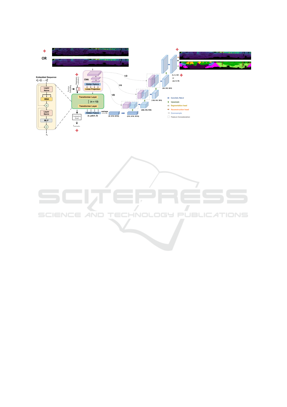
Figure 1: TransUnet architecture (Chen et al., 2021) extended to the self-training setting and used for sematic segmentation

of 2D spherical images projected from 3D point clouds in KITTI dataset (Geiger et al., 2012). The red star points to parts of

the architecture that exists only when self-training.

data augmentation or transformation is applied on the

training and validation sequences when funetuning.

As explained in Section 3.1, point cloud is pro-

jected on a spherical image of size 1024 × 64 and

processed by the network. When evaluation, the out-

put segmentation image is back projected to the point

cloud using k-Nearest-Neighbor (kNN) search (Mil-

ioto et al., 2019) to deﬁne the labels of the entire 3D

scan. Image of 2048×64 would have generated better

results but GPU dedicated memory wasn’t enough

4.2 Evaluation Metrics

For the semantic segmentation task, our goal

is to maximize the mean intersection of union

score (mIoU ) of the 20 classes represented in Se-

manticKITTI(Behley et al., 2019)(Geiger et al., 2012)

over the validation dataset.

Also the average PPNLL is compared for different

trained semantic segmentation models, to measure the

certainty i.e. how well the trained network can model

the true generation process of samples.

4.3 Results

4.3.1 Semantic Segmentation Results

Different models are obtained for different network

architectures:

• TransUnet architecture (Chen et al., 2021) Figure

• U-Net architecture Figure 3 b .

• TransUnet architecture (Chen et al., 2021) but

with replacing the CNN based encoder and de-

coder blocks with those used in SalsaNext archi-

tecture (Cortinhal et al., 2020) Figure 2.

• SalsaNext network implementation as (Cortinhal

et al., 2020).

Using one of the above architectures, we ﬁrst do self-

supervision training using either the reconstruction

loss plus the contrastive loss or only the reconstruc-

tion loss. Training dataset as in section 4.1 is used.

Pre-trained weight parameters are used to initialise

the segmentation network. Pre-training conﬁgura-

tions:

• Xavier (Glorot and Bengio, 2010) initialisation of

the segmentation network (a/A Figure 3).

• ImageNet (Deng et al., 2009) pre-trained weights

initialisation (a/B Figure 3).

• Xavier (Glorot and Bengio, 2010) initialisation

then self-training using the reconstruction loss

plus the contrastive loss (a/C Figure 3).

• ImageNet (Deng et al., 2009) pre-trained weights

initialisation then self-training using only the re-

construction loss (a/D Figure 3).

• Xavier (Glorot and Bengio, 2010) initialisation

then self-training using the reconstruction loss

only (a/E Figure 3).

• Xavier (Glorot and Bengio, 2010) initialisation

then self-training using the reconstruction loss

only. When ﬁne-tuning, Batch Normalisation lay-

ers are initialised using the Xavier (Glorot and

Bengio, 2010) (a/F Figure 3).

VISAPP 2022 - 17th International Conference on Computer Vision Theory and Applications

1014

Conv1

GN1 RELU

Conv2

GN2 RELU

Conv3

GN3

input

RELU

output

ResNet blockTransUnet

ResNet blockSalsaNext

Conv1

LRELU

BN1

Conv2

LRELU

BN2

Conv3

LRELU

BN3

Conv4

LRELU

BN4

CAT

Input

Dropout

Output

Decoder blockTransUnet

Conv1 BN1

RELU

2X CAT

Skip connection

Input

Conv2 BN2

RELU

Conv3 BN3

Output

Decoder blockSalsaNext

Dropout CAT Dropout

Skip connection

Conv1

LRELU

BN1 Conv2

LRELU

BN2

Conv3

LRELU

BN3CAT

Conv4

LRELU

BN4Dropout

Input

Output

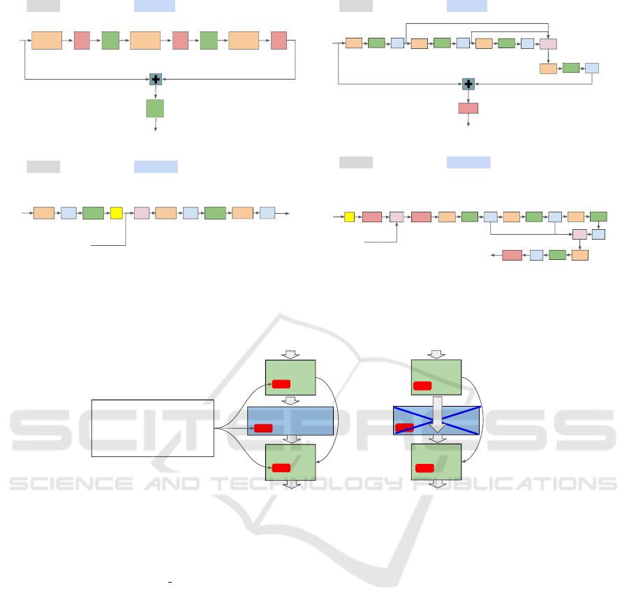
Figure 2: (Top) Architecture of the ResNet block in TransUnet (Chen et al., 2021) (left) and in SalsaNext (Cortinhal et al.,

2020) (right). (Bottom) Architecture of the Decoder block in TransUnet (Chen et al., 2021) (left) and in SalsaNext (Cortinhal

et al., 2020) (right). GN is Group Normalisation, BN is Batch Normalisation, CAT is concatenation layer, 2X is upsampling

by scale factor 2 and + is addition layer.

ENC

Transformer

DEC

input

Segmentation

Output

Skip

connections

A. Xavier-I

B. ImgNet-I

C. Xavier-I & Rec-Con-ST

D. ImgNet-I & Rec-ST

E. Xavier-I & Rec-ST

F. Xavier-I & Rec-ST & BN_R_I

ENC

Transformer

DEC

input

Segmentation

Output

Skip

connections

(a) (b)

Figure 3: Segmentation network initialised for different pre-training conﬁgurations. Xavier-i is Xavier initialisation, ImgNet-

i is ImageNet pre-trained weight initialisation, Rec-Con-ST is Reconstruction-Contrastive self-training, Rec-ST is Recon-

struction self-training and BN-R I is the Batch normalisation layers Xavier initialised, instead of the self-trained ones. (a)

TransUnet architecture. (b) U-Net architecture i.e.remove the Transformer.

The Segmentation network is either trained using the

Cross entropy loss or using the Cross entropy loss

plus the Lovasz-Softmax loss (L

+ L

). For any

of the 2 cases we don’t ignore any of the semantic

classes while training.

Semantic segmentation results are evaluated on

the validation dataset (without any data augmentation

or transformation) for different architectures, self-

training procedures and semantic segmentation train-

ing loss functions. mIoU score is shown for each self-

training and segementation training conﬁgurations in

Table 1. The results shows that,

• Self-training using reconstruction loss only, gen-

erates much higher mIoU (by highest difference =

2.9%) than using reconstruction plus contrastive

loss function.

• Adding the Transformer block to be a part of the

encoder in the U-Net architecture and doing self-

training improves the mIoU by +1.75% over U-

Net architecture only, even with self-training it too

Table 2.

• Self-training always improves the mIoU result,

where the highest improvement than training from

scratch is +2.28%.

• Initialising the segmentation model weight pa-

rameters using self-trained model for image

reconstruction objective generates better mIoU

(+0.48%) than initialising with pre-trained model

on ImageNet (Deng et al., 2009) for image classi-

ﬁcation training objective.

• Starting from Xavier (Glorot and Bengio, 2010)

Study of LiDAR Segmentation and Model’s Uncertainty using Transformer for Different Pre-trainings

1015

initialised weights then doing self-training with

image reconstruction objective, generates better

mIoU (by +0.47%) than starting from ImageNet

pre-trained weights and also doing self-training

with image reconstruction objective.

• Replacing the encoder and decoder blocks in Tan-

sUnet architecture (Chen et al., 2021) with those

in SalsaNext architecture (Cortinhal et al., 2020)

Figure 2 while keeping the self-training proce-

dure and the segmentation training loss function,

improves the mIoU by +11.86%, where there are

huge improvements in the jaccard index of classes

that are relatively small in size and not as repeated

in the dataset (person, bicycle...).

• Xavier (Glorot and Bengio, 2010) initialisation

of the Batch Normalisation layers instead of us-

ing the self-trained ones improves the mIoU by

+2.66%.

• Adding Lovasz-Softmax loss to the Cross entropy

loss function i.e.(L

) improves the mIoU by

+1.38% for the same architecture and same self-

training procedure.

• The best generated model outperforms SalsaNext

(Cortinhal et al., 2020) by +5.53% in the mIoU

score.

Also it’s observed that most of the time using the de-

coder block from the self-trained model generates bet-

ter mIoU (by ≈ 1.3%) than initialising it’s weights

using Xavier (Glorot and Bengio, 2010) in the seg-

mentation network. This is unlike what is mentioned

in (Studer et al., 2019).

4.3.2 Estimating Epistemic Uncertainty of

Different Models

The average PPNLL of the segmentation model is

evaluated over the validation dataset (without aug-

mentation or transformation) for different architec-

tures, self-training procedures and semantic segmen-

tation training loss functions. Dropout rate is 0.2 and

number of forward passes T=20. Mean pixel vali-

dation segmentation loss is evaluated using the nega-

tive log-likelihood loss (NLLLoss). Both the average

PPNLL and the validation segmentation loss are eval-

uated without ignoring any of the semantic classes.

We show the results in Table 3.

• For approximately the same mIoU score (1

and

rows in Table 3), the segmentation network

initialised using self-trained weights generates

less average PPNLL than the network initialised

using Xavier (Glorot and Bengio, 2010) which

mean less epistemic uncertainty.

• The model that achieves the lowest validation seg-

mentation loss also achieves the lowest average

negative predictive probability log-likelihood.

5 DISCUSSION

It was assumed that the task of the contrastive learn-

ing should allow better generalisation of the encoder

and Transformer networks Figure 1. To make sure it

was performed correctly, the contrastive learning was

validated through 1) randomly augmenting, z-axis ro-

tating and corrupting the validation dataset, 2) save

the contrastive embedding generated for each input

augmented image, 3) measure the distance between

the embedding of the input image (another differently

augmented version) to the saved embeddings, i.e. for

image index i, the output embedding should have the

closest distance to the saved embedding index i − 1 or

i or i + 1, in this case it is considered a match (as con-

secutive scans approximately cover the same scene

in KITTI (Geiger et al., 2012)). The matching accu-

racy score is 72%. Self-training using reconstruction

loss only is better than using reconstruction plus con-

trastive loss function.

This is because contrastive loss is a learning ob-

jective over the image level not the pixel level and

can beneﬁt the images discrimination but not segmen-

tation. Contrastive-Reconstruction self-training, but

this time the constrastvie loss over image patches as

(Chen et al., 2020), didn’t work. This can be rea-

soned that the patches across different images and

across the same image can be very similar for KITTI

dataset (Geiger et al., 2012), making the probability

of matching with the positive samples i.e. patches

from the same image, and the probability of match-

ing with the negative samples i.e. patches from dif-

ferent images both large values. Xavier (Glorot and

Bengio, 2010) initialisation of the Batch Normalisa-

tion layers is better than using the self-trained ones.

This is because when self-training, the parameters

of Batch Normalisation layers are learnt for the aug-

mented training dataset, not the original dataset which

is used for the semantic segmentation training.

Table 3, adding Lovasz-Softmax loss to the Cross

entropy loss function i.e.(L

) generated the best

mIoU score, yet the network’s output has large un-

certainty. The reason can be that the softmax output

score at the true class was the highest between other

classes yet with small margin. The SalsaNext (Cort-

inhal et al., 2020), generates the worst segmentation

validation loss and average PPNLL. This can be rea-

soned that, it ignores unlabeled pixels while training

which leads to miss-classifying them to other classes

VISAPP 2022 - 17th International Conference on Computer Vision Theory and Applications

1016

Table 1: Pre-trained models in the table (Figure 3 a) initialise the semantic segmentation network. mIoU scores in percent-

age. Scores are evaluated ignoring the unlabled class. Each sub-table represents different network architectures or different

segmentation training loss functions. Architecture or segmentation loss is same as predecessor sub-table unless mentioned

otherwise. Highest score in each section is in bold.

Pre-training conﬁgurations [section 4.3.1] mIoU

TransUnet (Chen et al., 2021), segmentation loss is Cross entropy

Xavier-I 34.28

ImageNet-I 36.08

Xavier-I & Rec-Con-ST 33.66

ImageNet-I & Rec-ST 36.09

Xavier-I & Rec-ST 36.56

Remove the Transformer from TransUnet (Chen et al., 2021)

Xavier-I & Rec-ST 34.81

TransUnet(Chen et al., 2021) replacing ENC & DEC with those in(Cortinhal et al., 2020)

Xavier-I 47.14

Xavier-I & Rec-ST 45.76

Xavier-I & Rec-ST & BN-R-I 48.42

Segmentation loss is Cross entropy + Lovasz-Softmax

Xavier-I & Rec-ST & BN-R I 49.8

SalsaNext (Cortinhal et al., 2020) using the authors’ implementation

Xavier-I 44.27

Table 2: Same as Table 1 but shows the Jaccard index for each class (except for the motorcyclist class as it’s Jaccard index

always 0) and mIoU score, all in percentage to show the improvements from integrating the Transformer into the U-Net

architecture. Higher score for each class is in bold.

Pre-training conﬁgurations [section 4.3.1]

Class

car

bicycle

motorcycle

truck

other-vehicle

person

bicyclist

road

parking

sidewalk

other-ground

building

fence

vegetation

trunk

terrain

pole

trafﬁc-sign

mIoU

TransUnet architecture (Chen et al., 2021). Segmentation loss is Cross entropy loss

Xavier-I & Rec-ST 20.13 12.21 11.33 50.01 23.67 17.01 22.14 91.64 27.29 74.01 0.33 77.93 37.36 79.79 38.92 66.58 44.27 0.1 36.56

TransUnet architecture (Chen et al., 2021) without the Transformer block. Segmentation loss is Cross entropy loss

Xavier-I & Rec-ST 19.86 8.25 12.46 30.65 20.94 13.08 28.76 91.33 27.78 73.78 0.03 77.02 32.6 79.69 33.12 68.43 43.47 0.1 34.81

Table 3: This table shows the average PPNLL results of different models. It tries to capture it’s relation to the mean validation

loss and the mIoU socre. Both the average PPNLL and the segmentation validation loss are evaluated (without ignoring any of

the semantic classes). The ﬁst 4 rows test the change in the average PPNLL result for 4 different model versions of the same

network architecture. The 5

row shows the results of the best generated model and the last row shows the results generated

after training SalsaNext (Cortinhal et al., 2020).

Pre-training conﬁgurations [section 4.3.1] mIoU (Table1) Mean segmentation validation loss Average predictive probability -ve log-likelihood

TransUnet architecture (Chen et al., 2021) with replacing the CNN based encoder and decoder blocks with those in (Cortinhal et al., 2020) Figure 2. Segmentation loss is Cross entropy loss

Xavier-I 47.14 0.283 2.985

Xavier-I & Rec-ST & BN-R I → mIoU score approx. equal above row 47 0.265 2.171

Xavier-I & Rec-ST & BN-R I → lowest mean segmentation validation loss for such architecture 46.18 0.256 1.951

Xavier-I & Rec-ST & BN-R I → Highest mIoU score for such architecture 48.42 0.268 2.445

TransUnet architecture (Chen et al., 2021) with replacing the encoder and decoder blocks with those in (Cortinhal et al., 2020) Figure 2. Segmentation loss is Cross entropy loss + Lovasz-Softmax loss (L

+ L

)

Xavier-I & Rec-ST & BN-R I 49.8 0.286 4.05

SalsaNext (Cortinhal et al., 2020) using the authors’ implementation and training settings

Xavier-I 44.27 2.782 85.523

while validation and increases the model’s epistemic

uncertainty.

6 CONCLUSIONS

Integrating the Transformer into the U-Net architec-

ture and doing self-training improves the mIoU by

+1.75% over U-Net architecture only, even with self-

training it too. Self-training using reconstruction loss

only results in much higher mIoU (by highest dif-

ference = 2.9%) than using reconstruction plus con-

trastive loss function.

Initialising the segmentation model weight param-

eters using self-trained model, results in higher mIoU

(+0.48%) than initialising with ImageNet pre-trained

model.

Study of LiDAR Segmentation and Model’s Uncertainty using Transformer for Different Pre-trainings

1017

Starting from Xavier initialised weights then do-

ing self-training, results in higher mIoU (by +0.47%)

than starting from ImageNet pre-trained weights and

also doing self-training. Still model initialisation us-

ing ImegeNet pre-trained weights outperforms Xavier

initialisation by 1.8% in the mIoU score.

Xavier initialisation of the Batch Normalisation

layers instead of using the self-trained ones improves

the mIoU by +2.66%.

Using the same machine, the same dataset and

same image input size (1024 × 64), our best gener-

ated model outperforms the SalsaNext by +5.53% in

the mIoU score. For approximately the same mIoU

score, the segmentation network initialised using self-

trained weights generates less average PPNLL than

the network initialised using Xavier. This shows that

self-training reduces the epistemic uncertainty of the

model. For the same architecture and same self-

training, the lower segmentation validation loss is, the

lower the model’s epistemic uncertainty.

The recipe that generated the best results was, us-

ing the TransUnet architecture, keep the Transformer

block but with replacing the CNN ResNet and de-

coder blocks with those in the SalsaNext architec-

ture, use the self-supervision training with input re-

construction objective, use the pre-trained weights to

initialise the segmentation network except the batch

normalisation layers which are randomly initialised

and use Cross entropy loss plus the Lovasz-Softmax

loss as the semantic segmentation loss.

REFERENCES

Assran, M., Caron, M., Misra, I., Bojanowski, P., Joulin, A.,

Ballas, N., and Rabbat, M. (2021). Semi-supervised

learning of visual features by non-parametrically pre-

dicting view assignments with support samples. arXiv

preprint arXiv:2104.13963.

Atito, S., Awais, M., and Kittler, J. (2021). Sit:

Self-supervised vision transformer. arXiv preprint

arXiv:2104.03602.

Balan, A. K., Rathod, V., Murphy, K., and Welling,

M. (2015). Bayesian dark knowledge. CoRR,

abs/1506.04416.

Behley, J., Garbade, M., Milioto, A., Quenzel, J., Behnke,

S., Stachniss, C., and Gall, J. (2019). SemanticKITTI:

A Dataset for Semantic Scene Understanding of Li-

DAR Sequences. In Proc. of the IEEE/CVF Interna-

tional Conf. on Computer Vision (ICCV).

Bhattacharyya, P., Huang, C., and Czarnecki, K. (2021). Sa-

det3d: Self-attention based context-aware 3d object

detection.

Caesar, H., Bankiti, V., Lang, A. H., Vora, S., Liong, V. E.,

Xu, Q., Krishnan, A., Pan, Y., Baldan, G., and Bei-

jbom, O. (2019). nuscenes: A multimodal dataset for

autonomous driving. CoRR, abs/1903.11027.

Carion, N., Massa, F., Synnaeve, G., Usunier, N., Kir-

illov, A., and Zagoruyko, S. (2020). End-to-end

object detection with transformers. arXiv preprint

arXiv:2005.12872.

Chen, H., Wang, Y., Guo, T., Xu, C., Deng, Y., Liu,

Z., Ma, S., Xu, C., Xu, C., and Gao, W. (2020).

Pre-trained image processing transformer. CoRR,

abs/2012.00364.

Chen, J., Lu, Y., Yu, Q., Luo, X., Adeli, E., Wangy, Y.,

Lu, L., Yuille, A. L., and Zhou, Y. (2021). Transunet:

Transformers make strong encoders for medical image

segmentation. arXiv preprint arXiv:2102.04306.

Cortinhal, T., Tzelepis, G., and Aksoy, E. E. (2020). Sal-

sanext: Fast, uncertainty-aware semantic segmenta-

tion of lidar point clouds for autonomous driving.

Dai, Z., Cai, B., Lin, Y., and Chen, J. (2021). Up-detr: Un-

supervised pre-training for object detection with trans-

formers. In Proceedings of the IEEE/CVF Conference

on Computer Vision and Pattern Recognition (CVPR),

pages 1601–1610.

Deng, J., Dong, W., Socher, R., Li, L.-J., Li, K., and Fei-

Fei, L. (2009). ImageNet: A Large-Scale Hierarchical

Image Database. In CVPR09.

Dosovitskiy, A., Beyer, L., Kolesnikov, A., Weissenborn,

D., Zhai, X., Unterthiner, T., Dehghani, M., Minderer,

M., Heigold, G., Gelly, S., Uszkoreit, J., and Houlsby,

N. (2021). An image is worth 16x16 words: Trans-

formers for image recognition at scale. In ICLR.

Gal, Y. and Ghahramani, Z. (2016). Dropout as a bayesian

approximation: Representing model uncertainty in

deep learning.

Geiger, A., Lenz, P., and Urtasun, R. (2012). Are we ready

for Autonomous Driving? The KITTI Vision Bench-

mark Suite. In Proc. of the IEEE Conf. on Computer

Vision and Pattern Recognition (CVPR), pages 3354–

3361.

Glorot, X. and Bengio, Y. (2010). Understanding the difﬁ-

culty of training deep feedforward neural networks. In

Teh, Y. W. and Titterington, M., editors, Proceedings

of the Thirteenth International Conference on Artiﬁ-

cial Intelligence and Statistics, volume 9 of Proceed-

ings of Machine Learning Research, pages 249–256,

Chia Laguna Resort, Sardinia, Italy. PMLR.

Graves, A. (2011). Practical variational inference for neural

networks. In Shawe-Taylor, J., Zemel, R., Bartlett,

P., Pereira, F., and Weinberger, K. Q., editors, Ad-

vances in Neural Information Processing Systems,

volume 24. Curran Associates, Inc.

Hahner, M., Dai, D., Liniger, A., and Gool, L. V. (2020).

Quantifying data augmentation for lidar based 3d ob-

ject detection. CoRR, abs/2004.01643.

Hao, W., Li, C., Li, X., Carin, L., and Gao, J. (2020).

Towards learning a generic agent for vision-and-

language navigation via pre-training. Conference on

Computer Vision and Pattern Recognition (CVPR).

Hern

andez-Lobato, J. M. and Adams, R. P. (2015). Prob-

abilistic backpropagation for scalable learning of

bayesian neural networks.

VISAPP 2022 - 17th International Conference on Computer Vision Theory and Applications

1018

Jaiswal, A., Babu, A. R., Zadeh, M. Z., Banerjee, D., and

Makedon, F. (2020). A survey on contrastive self-

supervised learning. CoRR, abs/2011.00362.

Lakshminarayanan, B., Pritzel, A., and Blundell, C. (2017).

Simple and scalable predictive uncertainty estimation

using deep ensembles.

Milioto, A., Vizzo, I., Behley, J., and Stachniss, C. (2019).

Rangenet++: Fast and accurate lidar semantic seg-

mentation. In Proc. of the IEEE/RSJ Intl. Conf. on

Intelligent Robots and Systems (IROS).

Minka, T. P. (2001). A family of algorithms for approximate

bayesian inference. In PhD thesis, Massachusetts In-

stitute of Technology.

Olaf Ronneberger, P. F. and Brox, T. (2015). U-net: Convo-

lutional networks for biomedical image segmentation.

arXiv preprint arXiv:1505.04597.

Qi, C. R., Su, H., Mo, K., and Guibas, L. J. (2017a). Point-

net: Deep learning on point sets for 3d classiﬁcation

and segmentation. In Proceedings of the IEEE con-

ference on computer vision and pattern recognition,

pages 652–660.

Qi, C. R., Yi, L., Su, H., and Guibas, L. J. (2017b). Point-

net++: Deep hierarchical feature learning on point sets

in a metric space. In Advances in neural information

processing systems, pages 5099–5108.

Qi, D., Su, L., Song, J., Cui, E., Bharti, T., and Sacheti,

A. (2020). Imagebert: Cross-modal pre-training with

large-scale weak-supervised image-text data. CoRR,

abs/2001.07966.

Studer, L., Alberti, M., Pondenkandath, V., Goktepe, P.,

Kolonko, T., Fischer, A., Liwicki, M., and Ingold,

R. (2019). A comprehensive study of imagenet

pre-training for historical document image analysis.

CoRR, abs/1905.09113.

Tchapmi, L. P., Choy, C. B., Armeni, I., Gwak, J., and

Savarese, S. (2017). Segcloud: Semantic segmenta-

tion of 3d point clouds. CoRR, abs/1710.07563.

Vaswani, A., Shazeer, N., Parmar, N., Uszkoreit, J., Jones,

L., Gomez, A. N., Kaiser, L., and Polosukhin, I.

(2017). Attention is all you need. In Advances in

neural information processing systems, pages 5998—

-6008.

Wu, Z., Xiong, Y., Stella, X. Y., and Lin, D. (2018). Unsu-

pervised feature learning via non-parametric instance

discrimination. In Proceedings of the IEEE Confer-

ence on Computer Vision and Pattern Recognition.

Zhao, H., Jiang, L., Jia, J., Torr, P. H. S., and Koltun, V.

(2020). Point transformer. CoRR, abs/2012.09164.

Zheng, S., Lu, J., Zhao, H., Zhu, X., Luo, Z., Wang, Y.,

Fu, Y., Feng, J., Xiang, T., Torr, P. H., and Zhang,

L. (2021). Rethinking semantic segmentation from a

sequence-to-sequence perspective with transformers.

In CVPR.

Zhou, Y. and Tuzel, O. (2017). Voxelnet: End-to-end learn-

ing for point cloud based 3d object detection. CoRR,

abs/1711.06396.

Study of LiDAR Segmentation and Model’s Uncertainty using Transformer for Different Pre-trainings

1019