Counting or Localizing? Evaluating Cell Counting and Detection in

Microscopy Images

Luca Ciampi

, Fabio Carrara

, Giuseppe Amato

and Claudio Gennaro

Institute of Information Science and Technologies, National Research Council, Pisa, Italy

Keywords:

Automatic Cell Counting, Biomedical Image Analysis, Deep Learning, Deep Learning for Visual

Understanding, Convolutional Neural Networks, Counting Objects in Images, Visual Counting.

Abstract:

Image-based automatic cell counting is an essential yet challenging task, crucial for the diagnosing of many

diseases. Current solutions rely on Convolutional Neural Networks and provide astonishing results. However,

their performance is often measured only considering counting errors, which can lead to masked mistaken

estimations; a low counting error can be obtained with a high but equal number of false positives and false

negatives. Consequently, it is hard to determine which solution truly performs best. In this work, we investigate

three general counting approaches that have been successfully adopted in the literature for counting several

different categories of objects. Through an experimental evaluation over three public collections of microscopy

images containing marked cells, we assess not only their counting performance compared to several state-of-

the-art methods but also their ability to correctly localize the counted cells. We show that commonly adopted

counting metrics do not always agree with the localization performance of the tested models, and thus we

suggest integrating the proposed evaluation protocol when developing novel cell counting solutions.

1 INTRODUCTION

Microscopy medical images analysis comprises sev-

eral challenging Computer Vision problems involving

a wide variety of tasks. Among them, cell localization

(Lugagne et al., 2019) and counting (Falk et al., 2018)

are essential steps for basic research, like disease di-

agnosis via the evaluation of cell growth kinetics, the

estimation of cytotoxicity (i.e., the quality of being

toxic to cells) (Kotoura et al., 1985), the quantiﬁcation

of perineuronal nets (Fawcett et al., 2019), the discov-

ery of the role of particular genes in cell biology, mi-

crobiology, and immunology (Zhang et al., 2015), and

many more. Manual cell counting is still conducted

in many laboratories, often with the aid of a hemocy-

tometer and its variants, which has been commonly

used due to its low cost and versatility (Johnston,

2010). However, the procedure is time-consuming

and error-prone, being subject to inter-user variation

depending on the degree of expertise of the analyst

(Altman et al., 1993). Therefore, there is a need to

https://orcid.org/0000-0002-6985-0439

https://orcid.org/0000-0001-5014-5089

https://orcid.org/0000-0003-0171-4315

https://orcid.org/0000-0002-3715-149X

count cells automatically to facilitate this tedious and

challenging task.

Recently, several vision models (mostly based on

Convolutional Neural Networks) have been success-

fully adopted to count cells and other biological struc-

tures from microscopy images. However, the per-

formance of these techniques is often measured only

considering the counting errors occurring at inference

time (i.e., the difference between the predicted and

the actual cell numbers), which often leads to masked

mistaken estimations. Indeed, counting errors do not

take into account where the cells have been local-

ized in the images and, consequently, counting mod-

els might achieve low values of errors while providing

wrong predictions (e.g., a high number of false posi-

tives and false negatives). Therefore, it is hard to per-

form a fair comparison between the different state-of-

the-art cell counting approaches to determine which

performs best.

In this work, we investigate three baseline

solutions belonging to the three main counting

methodologies — a segmentation-based approach, a

localization-based approach, and a count-density es-

timation approach — that have been successfully ex-

ploited for counting several different categories of ob-

jects, such as people and vehicles, and that repre-

Ciampi, L., Carrara, F., Amato, G. and Gennaro, C.

Counting or Localizing? Evaluating Cell Counting and Detection in Microscopy Images.

DOI: 10.5220/0010923000003124

In Proceedings of the 17th International Joint Conference on Computer Vision, Imaging and Computer Graphics Theory and Applications (VISIGRAPP 2022) - Volume 4: VISAPP, pages

887-897

ISBN: 978-989-758-555-5; ISSN: 2184-4321

887

sent the conceptual basis also for the cell counting

techniques. We conduct experiments on three public

datasets containing different cell types and character-

ized by distinct peculiarities. In addition to compar-

ing the performance of investigated methods against

state-of-the-art cell counters using established count-

ing evaluation metrics, we also measure the ability

of the models to localize the counted cells correctly.

Speciﬁcally, we adopt two additional metrics; a) the

Grid Average Mean absolute Error (GAME) metric,

a hybrid metric that simultaneously considers errors

in the object count and in their coarse location, and

b) the mean Average Precision (mAP), that summa-

rizes the cell precise localization performance. We

show that commonly adopted counting metrics (like

mean absolute error) do not always agree with the lo-

calization performance of the tested models, and thus

we suggest measuring both whenever possible to fa-

cilitate the practitioner in picking the most suitable

solution.

We organize the paper as follows. We review re-

lated work in Section 2. In Section 3, we describe

the datasets used for our experiments. Section 4 de-

scribes the investigated methodologies, while Sec-

tion 5 outlines the performed experiments and the ob-

tained results. Finally, Section 6 concludes the pa-

per. The code and the trained models are publicly

available at https://github.com/ciampluca/counting

perineuronal nets/tree/visapp-counting-cells.

2 RELATED WORKS

This section reviews some works concerning the

counting task in its generality and speciﬁcally tailored

to estimating the number of cells in microscopy im-

ages.

Visual Counting. The goal of the visual counting

task is to estimate the number of object instances

in still images or video frames (Lempitsky and Zis-

serman, 2010). Due to its interdisciplinary and

widespread applicability to many real-world applica-

tions, like calculating the number of people present

at an event (Boominathan et al., 2016), evaluating

the number of vehicles in urban scenarios (Ciampi

et al., 2021a), or counting animals in ecological

surveys (Arteta et al., 2016b), visual counting has

recently drawn the attention of researchers. Cur-

rent solutions address this task as a supervised deep

learning-based process. They fall into two main cat-

egories: counting by detection (Amato et al., 2019;

Amato et al., 2018; Laradji et al., 2018; Ciampi et al.,

2018) that requires prior detection or segmentation of

the single instances of objects, and counting by re-

gression (O

noro-Rubio and L

opez-Sastre, 2016; Li

et al., 2018; Ciampi et al., 2020; Ciampi et al., 2021b)

that instead tries to establish a direct mapping be-

tween the image features and the number of objects

in the scene, either directly or via the estimation of a

density map (i.e., a continuous-valued function). Re-

gression techniques have demonstrated superior per-

formance in crowded scenarios where the objects’ in-

stances are sometimes not well visible due to occlu-

sions and clumps. However, they cannot precisely lo-

calize the objects present in the scene, eventually pro-

viding only a coarse position of the area in which they

are distributed.

Microscope Cell Counting. Because of its

paramount importance, several cell counting deep

learning-based methods have been proposed in the

last years. They belong to both the detection-based

and the regression-based approaches, each having

the advantages and the drawbacks already discussed

above. A relevant example belonging to the for-

mer category is (Paulauskaite-Taraseviciene et al.,

2019), where authors exploited the popular Mask

R-CNN (He et al., 2017) instance segmentation

framework to detect overlapping cells. On the other

hand, a notable regression-based work is (Aich

and Stavness, 2018), where the authors regulated

activation maps from the ﬁnal convolutional layer of

the network by exploiting coarse ground-truth acti-

vation maps generated from simple dot annotations.

Authors in (Xie et al., 2016), instead, introduced a

CNN-based regression approach that maps the image

features with an associated density map, providing

also a coarse localization of the cells by ﬁnding

its peak values. Another example is represented

by (Segui et al., 2015), where the authors proposed a

regression-based technique and explored the features

that are learned to understand their underlying

representation. In (Cohen et al., 2017), another

regression-based deep neural network architecture

(named Count-ception) is presented, inspired by

the Inception family (Szegedy et al., 2015). More,

in (Guo et al., 2021), another density-based deep net-

work framework designed to solve the cell counting

task is introduced. Speciﬁcally, the authors propose

SAU-Net, extending the segmentation network U-

Net (Ronneberger et al., 2015) with a Self-Attention

module. Finally, in (He et al., 2021) the authors

exploited auxiliary CNNs to assist the training of the

intermediate layers of a density regressor. Hybrid

strategies have also been devised to deal with densely

concentrated cells but still generating individual cell

detections, such as (Falk et al., 2018; Xie et al.,

VISAPP 2022 - 17th International Conference on Computer Vision Theory and Applications

888

2018). These approaches ﬁrst generate intermediate

maps that indicate the likelihood of each pixel being

the center of a cell in the image. Then, they convert

these maps into detections by applying some form of

Non-Maximum Suppression (NMS).

Most of these works measure the counting perfor-

mance by computing the error between the predicted

and the actual cell number, hiding potentially mis-

taken localization. In this work, we consider three

general counting approaches on which cell-speciﬁc

techniques rely, and we also evaluate the quality of

the produced detections.

3 DATASETS

In this section, we describe the datasets employed in

this work, summarized in Table 1; in particular, we

consider three publicly available collections of mi-

croscopy images widely used in the context of the cell

counting task, presenting different peculiarities and

challenges.

3.1 VGG Cells Dataset

The VGG Cells dataset, introduced in (Lempitsky

and Zisserman, 2010), comprises 200 RGB highly-

realistic synthetic emulations of ﬂuorescence mi-

croscopy images of bacterial cells. Images have a

ﬁxed size of 256 × 256 × 3 pixels, and the cells are

clustered in speciﬁc regions and occluded with each

other. It is worth noting that the annotation procedure

is performed automatically and so labels are free of

errors. We show a sample of this dataset in Figure 1.

3.2 MBM Cells Dataset

The Modiﬁed Bone Marrow (MBM) Cells has been

initially collected by the authors of (Kainz et al.,

2015) from 11 RGB microscopy images (having a

ﬁxed size of 1200 × 1200 × 3 pixels) of the human

bone marrow tissues pertaining to 8 different pa-

tients. The marked cells belonging to this dataset

have a signiﬁcant shape variance; furthermore, non-

homogeneous tissue background makes their local-

ization more difﬁcult. In a subsequent work (Cohen

et al., 2017), the authors divided each image into four

patches of 600 × 600 × 3 pixels, for a total of 44 im-

ages. A sample of this dataset is reported in Figure 1.

3.3 Nuclei Cells Dataset

This dataset has been presented in (Sirinukunwattana

et al., 2016) and comprises 100 RGB microscopy

H&E stained histology images of colorectal adenocar-

cinomas having a common size of 500×500× 3. The

images refer to 9 different patients. They have been

cropped from non-overlapping areas representing a

variety of tissue appearances from normal and ma-

lignant regions. Still, they also comprise areas with

artifacts, over-staining, and failed autofocussing to

simulate realistic outliers. Another peculiarity of this

dataset is that the nuclei of the cells belong to four dif-

ferent categories, presenting different visual charac-

teristics; some experts have manually annotated them

by putting a dot over the centroids of each biologi-

cal structure for a total of 29,756 nuclei marked. In

the following, we refer to this dataset as Nuclei Cells

dataset. We report a sample of this dataset in Figure 1.

4 METHOD

We assume to have a labeled collection of N mi-

croscopy images X = {(I

), . . . , (I

)}, where

is the set of 2D-point annotations associated to the

i-th image I

. Each image has been manually anno-

tated by a human expert, and the annotations are in

the form of dots, i.e., coordinates localizing the cen-

troids of the cells present in the region of interest, as

is usually the case in the counting task.

We deﬁne a localization model f

as a Deep

Learning-based algorithm that takes as input an im-

age I and produces as output an associated set of co-

ordinates L = {p

, . . . , p

| p

∈ R

} localizing the

centroids of the cells to be counted. This model is

trained using location data X and can be implemented

following several different strategies; here, we test

three successful approaches from the literature, that

are segmentation, detection, and density estimation,

described below.

4.1 Foreground/Background

Segmentation

Proposed by (Falk et al., 2018), in this approach we

locate cells on the basis of a binary segmentation map

S ∈ {0, 1}

H×W

where ones represent pixels of objects

of interest, while zeros are considered background.

Each connected component in the segmentation map

represents a single object; the positions of the ob-

jects L are set to the coordinate of the centroids of

the connected components. As the implementation

of the model f

, we adopt the original U-Net archi-

tecture (Ronneberger et al., 2015) commonly used in

segmentation tasks. The model is trained to produce a

real-valued segmentation map

S = f

(I) ∈ [0, 1]

H×W

Counting or Localizing? Evaluating Cell Counting and Detection in Microscopy Images

889

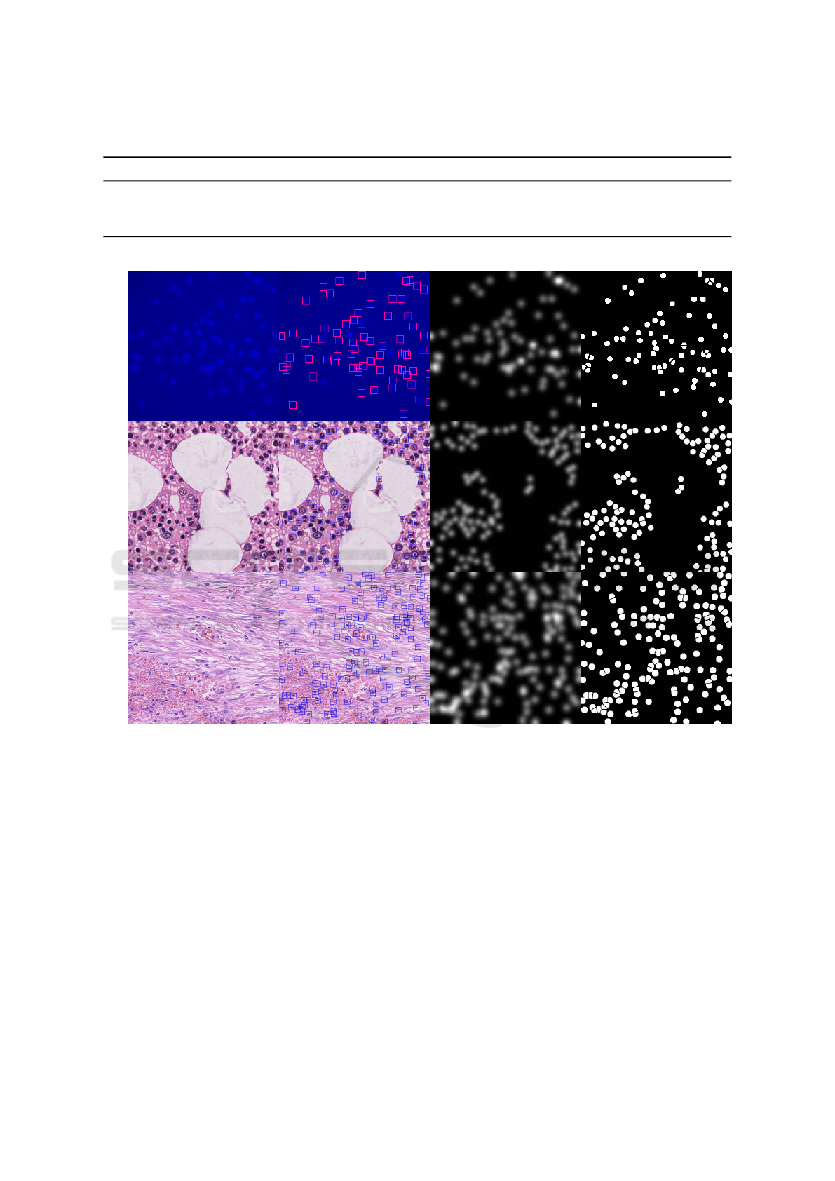
Table 1: Summary of datasets. We show the different peculiarities that characterize the three datasets exploited in this work.

Dataset N.Img Size N.Objs Objs/Img

VGG (Lempitsky and Zisserman, 2010) 200 256×256 35,192 176 ± 61

MBM (Kainz et al., 2015; Cohen et al., 2017) 44 600×600 5,553 126 ± 33

Nuclei (Sirinukunwattana et al., 2016) 100 500×500 29,756 297 ± 218

Sample Detection Target Density Target Segmentation Target

VGGMBM

Nuclei

Figure 1: Samples and Targets. We show a dataset sample (1

column) and the corresponding targets used when train-

ing i) the detection-based method FRCNN (2

column), ii) the density-based method D-CSRNet (3

column), and iii) the

segmentation-based method S-UNet (4

column).

that is then thresholded to obtain S. The target seg-

mentation maps are generated drawing discs at the

annotated positions and carefully separating overlap-

ping discs with a background ridge (see the fourth

column of Figure 1 for examples of targets). We min-

imize the weighted binary cross-entropy between pix-

els of the output and target maps as speciﬁed in (Falk

et al., 2018); more important pixels (near ridges and

foreground objects) are given an increased weight in

the total loss computation. We will refer to this ap-

proach as S-UNet.

4.2 Bounding Box Regression

For this approach, we employ the standard Faster-

RCNN detector (Ren et al., 2017). This deep neural

network takes images as input and produces a list of

bounding boxes localizing the objects as output. The

detection pipeline follows the two-stage paradigm. In

the ﬁrst stage, the network generates a bunch of re-

gion proposals likely to contain objects, exploiting a

set of anchors (i.e., pre-deﬁned boxes) that are sliced

over the image; in the second stage, these priors are

reﬁned and, for each of them, a score is assigned ex-

pressing the likelihood to really containing the object.

We consider the centers of the ﬁnal boxes as the lo-

VISAPP 2022 - 17th International Conference on Computer Vision Theory and Applications

890

calization of the entities we want to consider. We

produce the targets by generating squared bounding

boxes centered in the dot-annotated data and having

ﬁxed sides, again, depending on the typical object size

in the dataset. A sample of a target is shown in the

second column of Figure 1. We implement f

as a

Faster-RCNN network with a Feature Pyramid Net-

work module and a ResNet-50 backbone. From now

on, we will refer to this method as FRCNN.

4.3 Density Estimation

We also account for density-estimation approaches

that have shown superior counting performances in

very “crowded” scenarios. In this case, the goal is

to learn a regression between the features of an in-

put image having height H and width W to a density

map D = f

(I) ∈ R

H×W

. The notion of density map

is close to the physical/mathematical notion of den-

sity; speciﬁcally, each pixel of D corresponds to the

quantity of the objects present at that precise location.

The number of the objects n present in an image sub-

region P ⊆ I is estimated by summing up pixel val-

ues in the region of interest, i.e., n =

∑

p∈P

. Al-

though these approaches are not suited for precisely

localize objects, a coarse localization can be obtained

by analyzing the estimated density map, in particular

by ﬁnding the top-n maximum local peaks of it, as al-

ready done in (Xie et al., 2016). We train the model

by minimizing the mean squared error loss between

target and predicted density maps. Following previ-

ous works, we generate the target density maps by su-

perimposing Gaussian kernels G

centered in the dot-

annotated locations; the spread parameter σ is ﬁxed,

and it has been estimated depending on the typical

object size in the considered dataset. We show an

example of a target density map in the third column

of Figure 1. We implement f

exploiting the Con-

gested Scene Recognition Network (CSRNet), pro-

posed in (Li et al., 2018), a CNN for accurate den-

sity estimation of congested scenes, comprising two

major components. Speciﬁcally, it uses a modiﬁed

version of the popular VGG-16 network (Simonyan

and Zisserman, 2015) to extract the image features;

stacked upon this, the authors built a back-end com-

posed of dilated convolutional (Yu and Koltun, 2016)

layers to extract deeper information of saliency and,

at the same time, maintain the output resolution. We

will refer to this method as D-CSRNet.

5 EXPERIMENTS AND RESULTS

In this section, we describe the experiments per-

formed to validate our approach and discuss the ob-

tained results. First, we evaluate the three adopted

general counting solutions, i.e., the segmentation-

based S-UNet, the detection-based FRCNN, and the

density-based D-CSRNet approaches, over the three

standard cell counting benchmarks described above

to verify that the obtained counting errors are compa-

rable with the ones provided by state-of-the-art cell-

speciﬁc counting methods. Then, we perform addi-

tional experiments evaluating the quality of the local-

ization of the cells, an aspect that is not taken into

account by counting metrics.

5.1 Comparison with the

State-of-the-Art

We evaluate the three adopted counting methodolo-

gies over the VGG Cells, the MBM Cells, and the

Nuclei Cells counting benchmarks described in Sec-

tion 3, and we compare their performances with other

state-of-the-art approaches. For the VGG Cells and

the MBM Cells datasets, we follow the evaluation

protocol introduced by (Lempitsky and Zisserman,

2010) and adopted by most subsequent works. Specif-

ically, we consider a testing subset ﬁxed for all the

experiments (100 and 10 images for VGG Cells and

MBM Cells, respectively) and training and validation

subsets of varying size (N images for each subset) to

simulate lower or higher numbers of labeled exam-

ples. This evaluation protocol simulates the real sce-

nario in which scientists often have a signiﬁcant vari-

ance regarding the number of available microscopy

images. Following previous work, we set N to 16, 32,

and 50 for VGG Cells and to 5, 10, 15 for MBM Cells.

Concerning the Nuclei Cells dataset, we instead use

two-fold cross-validation, with 50 images for testing,

according to (Sirinukunwattana et al., 2016) and sub-

sequent works. Following standard counting bench-

marks, we use the Mean Absolute Error (MAE) to

measure the counting performance. Speciﬁcally, it is

deﬁned as:

MAE =

∑

n=1



− c

pred



, (1)

where N is the number of test images, c

is the ac-

tual count (i.e., the ground truth), and c

pred

is the pre-

dicted count of the n-th image. For the VGG Cells

and the MBM Cells, we repeat the experiment 10

times, randomly sampling ten different splits for each

conﬁguration, and we report the mean and standard

Counting or Localizing? Evaluating Cell Counting and Detection in Microscopy Images

891

deviation of the MAE computed between the differ-

ent runs. On the other hand, concerning the Nuclei

dataset, we report the mean and the standard devia-

tion of the MAE calculated between the 100 images

comprising the two test splits.

Table 2 reports the obtained results. The density-

based solution performs best among the VGG Cells

dataset and, more strongly, with the Nuclei Cells

dataset, comparably to the state of the art. The other

two adopted methods, i.e., the segmentation-based S-

UNet and the detection-based FRCNN, show larger

errors, according to their intrinsic limitations when

employed in highly “crowded” scenarios with oc-

cluded objects like the VGG Cells dataset and, espe-

cially, the Nuclei Cells dataset. On the other hand,

considering the MBM Cells dataset, characterized by

challenges more related to the object shape variations,

all the approaches show competitive results, in some

cases also outperforming state-of-the-art solutions.

5.2 Localization Analysis

Although the MAE is a fair metric for establishing a

comparative in terms of counting, it can often lead to

masking erroneous estimations. The reason is that the

MAE does not take into account where the estima-

tions have been done in the images. In other words,

the MAE does not capture localization errors; mod-

els might achieve low values of MAE while provid-

ing wrong predictions (e.g., a high number of false

positives and false negatives in detection-based tech-

niques, or a bad allocation of density values in pre-

dicted maps of density-based methods). Hence, pick-

ing up the best counting model basing the decision

only on the MAE metric can lead to blunders.

In this section, we conduct experiments to assess

the ability of the three adopted solutions to local-

ize the counted cells correctly. Speciﬁcally, we con-

sider two additional metrics described in the follow-

ing paragraphs.

Grid Average Mean absolute Error (GAME).

(Guerrero-G

omez-Olmedo et al., 2015) is a hybrid

metric that simultaneously considers the object count

and the estimated locations of the cells. Speciﬁ-

cally, it is computed by sub-dividing the image in 4

non-overlapping regions and summing the MAE com-

puted in each of these sub-regions. Formally:

GAME(L) =

∑

n=1

(

∑

l=1

− c

pred

|), (2)

where N is the total number of test images, c

pred

is the

estimated count in a region l of the n-th image, and

is the ground truth for the same region in the same

image. The higher L, the more restrictive the GAME

metric will be. Note that the MAE can be obtained as

a particular case of the GAME when L = 0.

Mean Average Precision (mAP). is an established

metric for the localization performances of object de-

tectors. We compute the average precision for an im-

age as follows. i) We assign a score to each detected

cell in the image. Detection scores are obtained dif-

ferently for the three tested methods. For the S-UNet

model, the detection score of an object is set to the

value of the predicted segmentation map

S at the lo-

cation of the centroid of the corresponding connected

component. For D-CSRNet, the location of an object

is set to a local peak in the predicted density map, and

its score is set to the value at its location. For FR-

CNN, the detection score is already part of the output

of the Faster-RCNN model. ii) We ﬁlter out weak

detections using a threshold on the detection scores.

iii) We match the ﬁltered detections with the ground-

truth object positions using the Hungarian algorithm

with a constraint on the maximum accepted displace-

ment in pixels between predicted and real locations;

once matches are found, we obtain the number of true

positives (matched detection and ground-truth pairs),

false positives (unmatched detections), and false neg-

atives (unmatched ground-truth positions) locations.

iv) We repeat these steps for several threshold values

to obtain the precision-recall curve and the average

precision (i.e., the area under the curve).

In Table 3, we report the MAE, the GAME, and

the mAP metrics for all the tested solutions and the

adopted datasets. Here, we consider only the splits

having N to 50 and 15 for the VGG and the MBM

datasets, respectively, and the same two-fold cross-

validation with 50 images for testing concerning the

Nuclei dataset. Note that the density-based solution

D-CSRNet shines in the Nuclei benchmark where

very dense regions of overlapped cells are common

and strain non-density solutions, obtaining the best

counting metrics (MAE, GAME) among the tested

models. However, the denser the cells in the bench-

mark, the less the density-based solution can recover

the exact locations of the counted cells, thus achieving

lower mAP values. On the other hand, the detection-

based solution FRCNN performs sufﬁciently well

only when counting cells in the less crowded MBM

and VGG benchmarks. Still, it is able to recover

the exact position of more counted cells, as can be

seen from the higher mAP values obtained. Last, the

segmentation-based model sits in the middle of these

two extremes, providing intermediate counting and

localization performance.

VISAPP 2022 - 17th International Conference on Computer Vision Theory and Applications

892

Table 2: Comparison on Standard Benchmarks. For VGG and MBM datasets, we vary the training and validation subsets

(N images for each subset), repeating the experiments 10 times. For Nuclei, we perform 2-fold cross-validation (N = 50

images per fold). Mean±st.dev. of MAE is reported.

VGG Cells (Lempitsky and Zisserman, 2010). (200 images in total - 100 test images)

Method N = 16 N = 32 N = 50

(Arteta et al., 2016a) N/A 5.06 ± 0.2 N/A

GMN (Lu et al., 2019) N/A 3.6 ± 0.3 N/A

(Lempitsky and Zisserman, 2010) 3.8 ± 0.2 3.5 ± 0.2 N/A

VGG-GAP-HR (Aich and Stavness, 2018)

∗

N/A 2.95

∗∗

2.67

SAU-Net (Guo et al., 2021) N/A N/A 2.6 ± 0.4

†

FCRN-A (Xie et al., 2016) 3.4 ± 0.2 2.9 ± 0.2 2.9 ± 0.2

‡

Count-Ception (Cohen et al., 2017) 2.9 ± 0.5 2.4 ± 0.4 2.3 ± 0.4

CCF (Jiang and Yu, 2020) 2.8 ± 0.1 2.6 ± 0.1 2.6 ± 0.1

C-FCRN+Aux (He et al., 2021) 2.3 ± 2.2

S-UNet (Falk et al., 2018) 8.3 ± 2.3 5.6 ± 1.1 4.5 ± 0.5

D-CSRNet (Li et al., 2018) 4.0 ± 0.2 3.2 ± 0.2 3.0 ± 0.1

FRCNN (Ren et al., 2017) 9.3 ± 0.7 8.2 ± 0.6 7.4 ± 1.0

* They did not report standard deviation. ** They used a validation subet of 100− N images. † They did not use a test

subset, but only a 100 − N images validation subset. ‡ Reported in their work as N = 64. $ They used a 5-fold cross

validation-based evaluation protocol considering the whole dataset.

MBM Cells (Kainz et al., 2015; Cohen et al., 2017). (44 images in total - 10 test images)

Method N = 5 N = 10 N = 15

(Xie et al., 2018) 36.3 ± 19.4

FCRN-A (Xie et al., 2016) 28.9 ± 22.6 22.2 ± 11.6 21.3 ± 9.4

(Marsden et al., 2018)

∗

23.6 ± 4.6 21.5 ± 4.2 20.5 ± 3.5

Count-Ception (Cohen et al., 2017) 12.6 ± 3.0 10.7 ± 2.5 8.8 ± 2.3

CCF (Jiang and Yu, 2020)

∗

9.3 ± 1.4 8.9 ± 0.9 8.6 ± 0.3

C-FCRN+Aux (He et al., 2021) 6.5 ± 5.2

∗∗

SAU-Net (Guo et al., 2021) N/A N/A 5.7 ± 1.2

†

S-UNet (Falk et al., 2018) 9.0 ± 1.9 7.0 ± 1.6 6.7 ± 2.5

D-CSRNet (Li et al., 2018) 10.8 ± 2.5 8.0 ± 1.3 7.0 ± 1.3

FRCNN (Ren et al., 2017) 8.8 ± 1.4 9.9 ± 1.5 8.3 ± 1.9

* They used 14 test images. ** They used a 5-fold cross validation-based evaluation protocol considering the whole dataset.

† They did not use a test subset, but only a 44 − N images validation subset.

They used a train/test split of 8/3 using

full-size images.

Nuclei Cells (Sirinukunwattana et al., 2016). (100 images in total - 50 test images)

Method N = 50

DeepFeat (Segui et al., 2015) 71.8 ± 51.4

(Lempitsky and Zisserman, 2010) 51.4 ± 39.8

StructRegNet (Xie et al., 2018) 45.9 ± 47.9

FCRN-A (Xie et al., 2016) 42.5 ± 33.5

Count-Ception (Cohen et al., 2017) 34.1 ± 29.0

C-FCRN+Aux (He et al., 2021) 29.3 ± 25.4

S-UNet (Falk et al., 2018) 62.4 ± 55.4

D-CSRNet (Li et al., 2018) 37.3 ± 41.0

FRCNN (Ren et al., 2017) 96.5 ± 128.0

Counting or Localizing? Evaluating Cell Counting and Detection in Microscopy Images

893

Table 3: Counting and Localization Performance. The MAE measures global counting performance independently of lo-

calization. The mAP summarizes localization performances in terms of precision and recall of localized cells. The GAME(L)

measure counting performance while being aware of the location of cells; the higher L, the more localization errors are penal-

ized. Regarding the VGG and the MBM datasets, we consider the splits having N to 50 and 15, respectively.

VGG Cells (Lempitsky and Zisserman, 2010). (200 images in total - 100 test images)

GAME(L) ↓

Method MAE ↓ L = 1 L = 2 L = 3 L = 4 mAP (%) ↑

S-UNet 4.5 ± 0.5 7.7 ± 1.3 12.8 ± 1.5 21.6 ± 2.4 38.0 ± 4.1 75.3 ± 15.8

D-CSRNet 3.0 ± 0.1 6.5 ± 0.2 11.3 ± 0.4 18.9 ± 0.6 28.7 ± 1.0 43.2 ± 1.6

FRCNN 7.4 ± 1.0 11.1 ± 0.9 18.3 ± 1.3 29.7 ± 2.0 43.3 ± 3.2 93.3 ± 0.6

MBM Cells (Kainz et al., 2015; Cohen et al., 2017). (44 images in total - 10 test images)

GAME(L) ↓

Method MAE ↓ L = 1 L = 2 L = 3 L = 4 mAP (%) ↑

S-UNet 6.7 ± 2.5 10.4 ± 2.5 17.3 ± 1.9 27.6 ± 2.0 40.9 ± 3.1 53.5 ± 5.3

D-CSRNet 7.0 ± 1.3 10.8 ± 1.2 16.7 ± 1.3 27.0 ± 1.6 41.5 ± 2.2 67.9 ± 1.2

FRCNN 8.3 ± 1.9 12.7 ± 2.4 20.4 ± 3.9 32.5 ± 4.7 47.2 ± 8.7 87.4 ± 1.9

Nuclei Cells (Sirinukunwattana et al., 2016). (100 images in total - 50 test images)

GAME(L) ↓

Method MAE ↓ L = 1 L = 2 L = 3 L = 4 mAP (%) ↑

S-UNet 62.4 ± 55.4 66.9 ± 51.7 75.1 ± 50.6 95.3 ± 54.1 138.4 ± 75.2 66.8 ± 11.7

D-CSRNet 37.3 ± 41.0 45.7 ± 38.8 58.2 ± 38.5 77.6 ± 39.8 100.5 ± 45.0 27.7 ± 8.5

FRCNN 96.5 ± 128.0 103.8 ± 125.3 112.6 ± 121.9 133.9 ± 118.7 168.2 ± 123.2 57.9 ± 10.8

Finally, in Figure 2, we show some examples of

predictions with very low absolute counting errors

(suggesting good performance) but in which the aver-

age precision metric indicates erroneous predictions

instead. Note that in the detection-based solution

FRCNN, the disagreement between the two metrics

is less pronounced, as this methodology is usually

adopted to optimize AP. Thus, we suggest integrat-

ing the mean average precision, or at least a GAME-

L metric with a high-enough L, when optimizing and

evaluating novel cell counting solutions. We deem the

additional evaluation protocol would help practition-

ers to better characterize the performance of devel-

oped solutions.

6 CONCLUSIONS

In this work, we consider the cell counting task in

microscopy images, investigating the ability of three

general counting methodologies not only in estimat-

ing the number of the biological structures but also

in localizing them. Indeed, most state-of-the-art so-

lutions tailored to cell counting are evaluated merely

considering the difference between the predicted and

the actual number of the cells, skipping a further anal-

ysis focused on the quality of the provided estima-

tions. We show that relying only on the counting met-

rics can lead to models producing incorrect cell lo-

calization. We performed experiments on three cell

counting benchmarks, and we assessed that counting

errors do not always agree with the localization per-

formance. Thus, we suggest measuring and reporting

also the mean average precision (or at least a grid av-

erage mean absolute error) whenever possible to help

practitioners developing better models and to guide

users to choose the model most tailored to their sce-

nario.

ACKNOWLEDGEMENTS

This work was partially funded by: AI4Media -

A European Excellence Centre for Media, Society

and Democracy (EC, H2020 n. 951911), Exten-

sion (ESA, n. 4000132621/20/NL/AF), and AI-MAP

(CNR4C program) - Tuscany POR FSE 2014-2020

(CUP B15J19001040004).

VISAPP 2022 - 17th International Conference on Computer Vision Theory and Applications

894

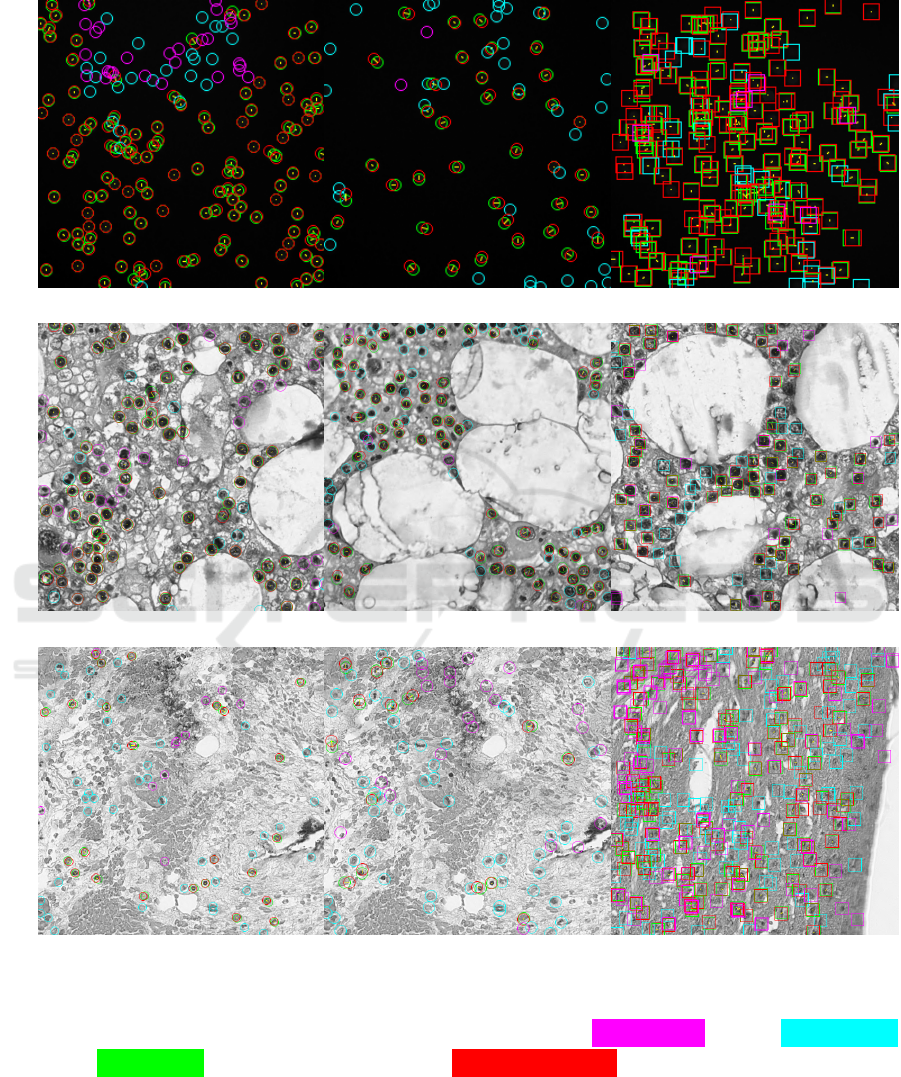
S-UNet D-CSRNet FRCNN

VGG

AE = 0 AP = 36.9% AE = 2 AP = 50.8% AE = 0 AP = 88.3%

MBM

AE = 1 AP = 34.3% AE = 3 AP = 61.9% AE = 0 AP = 79.1%

Nuclei

AE = 4 AP = 36.7% AE = 1 AP = 17.4% AE = 2 AP = 43.3%

Figure 2: Absolute Error (AE) can be misleading. For each considered model (one per column), we show predictions

obtaining a low AE, but also a low Average Precision (AP) due to high numbers of false positive and false negatives. The AP

can discern cases where the MAE fails to capture poor model outputs. We indicate false positives in purple, false negatives

in cyan, and true positives in green, with the corresponding ground-truth position drawn in red and connected via a thin

yellow line. (Best viewed in electronic format.)

Counting or Localizing? Evaluating Cell Counting and Detection in Microscopy Images

895

REFERENCES

Aich, S. and Stavness, I. (2018). Improving object counting

with heatmap regulation. CoRR, abs/1803.05494.

Altman, S. A., Randers, L., and Rao, G. (1993). Com-

parison of trypan blue dye exclusion and ﬂuorometric

assays for mammalian cell viability determinations.

Biotechnology Progress, 9(6):671–674.

Amato, G., Bolettieri, P., Moroni, D., Carrara, F., Ciampi,

L., Pieri, G., Gennaro, C., Leone, G. R., and Vairo, C.

(2018). A wireless smart camera network for parking

monitoring. In 2018 IEEE Globecom Workshops (GC

Wkshps), pages 1–6. IEEE.

Amato, G., Ciampi, L., Falchi, F., and Gennaro, C. (2019).

Counting vehicles with deep learning in onboard UAV

imagery. In 2019 IEEE Symposium on Computers and

Communications (ISCC), pages 1–6. IEEE.

Arteta, C., Lempitsky, V., Noble, J. A., and Zisserman,

A. (2016a). Detecting overlapping instances in mi-

croscopy images using extremal region trees. Medical

Image Analysis, 27:3–16.

Arteta, C., Lempitsky, V. S., and Zisserman, A. (2016b).

Counting in the wild. In Computer Vision - ECCV

2016, volume 9911, pages 483–498. Springer.

Boominathan, L., Kruthiventi, S. S. S., and Babu, R. V.

(2016). Crowdnet: A deep convolutional network for

dense crowd counting. In Proceedings of the 24th

ACM international conference on Multimedia, pages

640–644. ACM.

Ciampi, L., Amato, G., Falchi, F., Gennaro, C., and Ra-

bitti, F. (2018). Counting vehicles with cameras.

In Bergamaschi, S., Noia, T. D., and Maurino, A.,

editors, Proceedings of the 26th Italian Symposium

on Advanced Database Systems, Castellaneta Marina

(Taranto), Italy, June 24-27, 2018, volume 2161 of

CEUR Workshop Proceedings. CEUR-WS.org.

Ciampi, L., Gennaro, C., Carrara, F., Falchi, F., Vairo, C.,

and Amato, G. (2021a). Multi-camera vehicle count-

ing using edge-ai. CoRR, abs/2106.02842.

Ciampi, L., Santiago, C., Costeira, J., Gennaro, C., and Am-

ato, G. (2021b). Domain adaptation for trafﬁc den-

sity estimation. In Proceedings of the 16th Interna-

tional Joint Conference on Computer Vision, Imag-

ing and Computer Graphics Theory and Applications,

pages 185–195. SCITEPRESS - Science and Technol-

ogy Publications.

Ciampi, L., Santiago, C., Costeira, J. P., Gennaro, C., and

Amato, G. (2020). Unsupervised vehicle counting

via multiple camera domain adaptation. In Safﬁotti,

A., Seraﬁni, L., and Lukowicz, P., editors, Proceed-

ings of the First International Workshop on New Foun-

dations for Human-Centered AI (NeHuAI) co-located

with 24th European Conference on Artiﬁcial Intelli-

gence (ECAI 2020), Santiago de Compostella, Spain,

September 4, 2020, volume 2659 of CEUR Workshop

Proceedings, pages 82–85. CEUR-WS.org.

Cohen, J. P., Boucher, G., Glastonbury, C. A., Lo, H. Z.,

and Bengio, Y. (2017). Count-ception: Counting by

fully convolutional redundant counting. In 2017 IEEE

International Conference on Computer Vision Work-

shops (ICCVW), pages 18–26. IEEE.

Falk, T., Mai, D., Bensch, R.,

Ozg

un C¸ ic¸ek, Abdulkadir,

A., Marrakchi, Y., B

ohm, A., Deubner, J., J

ackel, Z.,

Seiwald, K., Dovzhenko, A., Tietz, O., Bosco, C. D.,

Walsh, S., Saltukoglu, D., Tay, T. L., Prinz, M., Palme,

K., Simons, M., Diester, I., Brox, T., and Ronneberger,

O. (2018). U-net: deep learning for cell counting, de-

tection, and morphometry. Nat. Methods, 16(1):67–

70.

Fawcett, J. W., Oohashi, T., and Pizzorusso, T. (2019). The

roles of perineuronal nets and the perinodal extracel-

lular matrix in neuronal function. Nat. Rev. Neurosci.,

20(8):451–465.

Guerrero-G

omez-Olmedo, R., Torre-Jim

enez, B., L

opez-

Sastre, R., Maldonado-Basc

on, S., and O

noro-Rubio,

D. (2015). Extremely overlapping vehicle counting. In

Pattern Recognition and Image Analysis, pages 423–

431. Springer International Publishing.

Guo, Y., Krupa, O., Stein, J., Wu, G., and Krishnamurthy,

A. (2021). SAU-net: A uniﬁed network for cell count-

ing in 2d and 3d microscopy images. IEEE/ACM

Trans. Comput. Biol. Bioinform., pages 1–1.

He, K., Gkioxari, G., Doll

ar, P., and Girshick, R. (2017).

Mask r-cnn. In Proceedings of the IEEE international

conference on computer vision, pages 2961–2969.

He, S., Minn, K. T., Solnica-Krezel, L., Anastasio, M. A.,

and Li, H. (2021). Deeply-supervised density regres-

sion for automatic cell counting in microscopy im-

ages. Medical Image Analysis, 68:101892.

Jiang, N. and Yu, F. (2020). A cell counting framework

based on random forest and density map. Appl. Sci.,

10(23):8346.

Johnston, G. (2010). Automated handheld instrument im-

proves counting precision across multiple cell lines.

BioTechniques, 48(4):325–327.

Kainz, P., Urschler, M., Schulter, S., Wohlhart, P., and Lep-

etit, V. (2015). You should use regression to detect

cells. In Lecture Notes in Computer Science, pages

276–283. Springer International Publishing.

Kotoura, Y., Yamamuro, T., Shikata, J., Kakutani, Y., Kit-

sugi, T., and Tanaka, H. (1985). A method for toxi-

cological evaluation of biomaterials based on colony

formation of v79 cells. Archives of Orthopaedic and

Traumatic Surgery, 104(1):15–19.

Laradji, I. H., Rostamzadeh, N., Pinheiro, P. O., Vazquez,

D., and Schmidt, M. (2018). Where are the blobs:

Counting by localization with point supervision. In

Computer Vision – ECCV 2018, volume 11206, pages

560–576. Springer International Publishing.

Lempitsky, V. S. and Zisserman, A. (2010). Learning to

count objects in images. In Advances in Neural Infor-

mation Processing Systems 23: 24th Annual Confer-

ence on Neural Information Processing Systems 2010,

pages 1324–1332. Curran Associates, Inc.

Li, Y., Zhang, X., and Chen, D. (2018). CSRNet: Dilated

convolutional neural networks for understanding the

highly congested scenes. In 2018 IEEE/CVF Con-

ference on Computer Vision and Pattern Recognition,

pages 1091–1100. IEEE.

Lu, E., Xie, W., and Zisserman, A. (2019). Class-agnostic

VISAPP 2022 - 17th International Conference on Computer Vision Theory and Applications

896

counting. In Computer Vision – ACCV 2018, pages

669–684. Springer International Publishing.

Lugagne, J.-B., Lin, H., and Dunlop, M. J. (2019). DeLTA:

Automated cell segmentation, tracking, and lineage

reconstruction using deep learning.

Marsden, M., McGuinness, K., Little, S., Keogh, C. E., and

O'Connor, N. E. (2018). People, penguins and petri

dishes: Adapting object counting models to new vi-

sual domains and object types without forgetting. In

2018 IEEE/CVF Conference on Computer Vision and

Pattern Recognition. IEEE.

noro-Rubio, D. and L

opez-Sastre, R. J. (2016). Towards

perspective-free object counting with deep learning.

In Computer Vision – ECCV 2016, volume 9911,

pages 615–629. Springer International Publishing.

Paulauskaite-Taraseviciene, A., Sutiene, K., Valotka, J.,

Raudonis, V., and Iesmantas, T. (2019). Deep

learning-based detection of overlapping cells. In Pro-

ceedings of the 2019 3rd International Conference on

Advances in Artiﬁcial Intelligence, pages 217–220.

ACM.

Ren, S., He, K., Girshick, R., and Sun, J. (2017). Faster r-

CNN: Towards real-time object detection with region

proposal networks. IEEE Trans. Pattern Anal. Mach.

Intell., 39(6):1137–1149.

Ronneberger, O., Fischer, P., and Brox, T. (2015). U-

net: Convolutional networks for biomedical image

segmentation. In Medical Image Computing and

Computer-Assisted Intervention - MICCAI 2015, vol-

ume 9351 of Lecture Notes in Computer Science,

pages 234–241. Springer.

Segui, S., Pujol, O., and Vitria, J. (2015). Learning to count

with deep object features. In 2015 IEEE Conference

on Computer Vision and Pattern Recognition Work-

shops (CVPRW). IEEE.

Simonyan, K. and Zisserman, A. (2015). Very deep convo-

lutional networks for large-scale image recognition. In

3rd International Conference on Learning Represen-

tations, ICLR 2015.

Sirinukunwattana, K., Raza, S. E. A., Tsang, Y.-W., Snead,

D. R. J., Cree, I. A., and Rajpoot, N. M. (2016). Lo-

cality sensitive deep learning for detection and clas-

siﬁcation of nuclei in routine colon cancer histol-

ogy images. IEEE Transactions on Medical Imaging,

35(5):1196–1206.

Szegedy, C., Liu, W., Jia, Y., Sermanet, P., Reed, S.,

Anguelov, D., Erhan, D., Vanhoucke, V., and Rabi-

novich, A. (2015). Going deeper with convolutions. In

2015 IEEE Conference on Computer Vision and Pat-

tern Recognition (CVPR), pages 1–9. IEEE.

Xie, W., Noble, J. A., and Zisserman, A. (2016). Mi-

croscopy cell counting and detection with fully con-

volutional regression networks. Comput. methods

Biomech. Biomed. Eng. Imaging Vis., 6(3):283–292.

Xie, Y., Xing, F., Shi, X., Kong, X., Su, H., and Yang, L.

(2018). Efﬁcient and robust cell detection: A struc-

tured regression approach. Medical Image Analysis,

44:245–254.

Yu, F. and Koltun, V. (2016). Multi-scale context aggre-

gation by dilated convolutions. In 4th International

Conference on Learning Representations, ICLR 2016.

Zhang, F., Qian, X., Si, H., Xu, G., Han, R., and Ni, Y.

(2015). Signiﬁcantly improved solvent tolerance of

escherichia coli by global transcription machinery en-

gineering. Microbial Cell Factories, 14(1).

Counting or Localizing? Evaluating Cell Counting and Detection in Microscopy Images

897