Discussion on Comparing Machine Learning Models

for Health Outcome Prediction

Janusz Wojtusiak

and Negin Asadzadehzanjani

Health Informatics Program, Department of Health Administration and Policy,

George Mason University, Fairfax, VA, U.S.A.

Keywords: Machine Learning, Health Data, Model Comparison.

Abstract: This position paper argues the need for more details than simple statistical accuracy measures when comparing

machine learning models constructed for patient outcome prediction. First, statistical accuracy measures are

briefly discussed, including AROC, APRC, predictive accuracy, precision, recall, and their variants. Then,

model correlation plots are introduced that compare outputs from two models. Finally, a more detailed

analysis of inputs to the models is presented. The discussions are illustrated with two classification problems

in predicting patient mortality and high utilization of medical services.

1 INTRODUCTION

There is a significant recent growth in the use of

Machine Learning (ML) methods in medical,

healthcare and health applications. These applications

span from patient risk stratification (Tseng et al.,

2020; Beaulieu-Jones et al., 2021), to differential

diagnosis (Castellazzi et al., 2020; Vaccaro et al.,

2021), to image recognition and analysis (Rahane et

al., 2018; Saha et al. 2021). The application of ML

methods achieved incredible results that often

outperform human experts. This growing interest is

followed by strong opposition to the use of ML and

criticism of the methods. Among the most often cited

criticisms are lack of reproducibility of results

(McDermott et al., 2021), biases in constructed

models, sometimes referred to as lack of fairness

(Mehrabi, 2021), and lack of transparency.

The context of the presented work is supervised

learning from medical or health data applied to

prediction of patient outcomes. Such data can consist

of medical claims, electronic medical records,

registries, surveys, and all other types of data, but can

be applied beyond healthcare. In our 2021

HEALTHINF presentation (Wojtusiak, 2021), we

argued the need for detailed reporting of results when

presenting outcomes of ML modeling of health-

related problems. That work identified ten MLI

https://orcid.org/0000-0003-2238-0588

criteria for reporting results: (1) experimental design,

(2) statistical model evaluation, (3) model calibration,

(4) top predictors, (5) global sensitivity analysis, (6)

decision curve analysis, (7) global model explanation,

(8) local prediction explanation, (9) programming

interface and (10) source code. Although not always

sufficient, these criteria are argued to be necessary to

describe constructed models and allow for

reproducibility of results.

Different questions arise when one needs to

compare two or more models. Is it sufficient to

compare models based on their performance

(accuracy) only? Should one use all of the above

ten criteria to compare models? Are some

additional tests needed to understand differences

between models? And most importantly: what does

it actually mean that one model is better than

another?

There is surprisingly little literature that present

frameworks for comparing ML models. When

searching for published works on comparison of ML

models, all papers that appear are comparing specific

models (or algorithms) for solving specific problems

at hand. Virtually all of them report only some

statistical measures discussed here in Section 3.

Similarly, large number of “data science” websites

discuss practical aspects of comparing models,

including examples of source code, but also limit

these comparisons to statistical accuracy measures.

Wojtusiak, J. and Asadzadehzanjani, N.

Discussion on Comparing Machine Learning Models for Health Outcome Prediction.

DOI: 10.5220/0010916600003123

In Proceedings of the 15th International Joint Conference on Biomedical Engineering Systems and Technologies (BIOSTEC 2022) - Volume 5: HEALTHINF, pages 711-718

ISBN: 978-989-758-552-4; ISSN: 2184-4305

711

There are approaches available in other fields. Lee

and Sangiovanni-Vincentelli (1998) presented a

general framework for comparing computation

methods. While their work is applicable to the

problems presented here, they do not provide

practical insights.

The concepts presented in this paper are described

in context of classification learning problems, and

most often binary classification, but can be

generalized to multiclass problems as well as

regression.

The discussed approaches are illustrated in terms

of two supervised learning problems, which are

constructed to predict patient outcomes using medical

claims data. More specifically, medical claims for

five percent control set of the linked Medicare

beneficiaries from the Surveillance, Epidemiology,

and End Results (SEER)-Medicare dataset between

1995 and 2013 were used to construct the models.

The Medicare claims collected by Medicare and

Medicaid Services (CMS) provide one of the largest

longitudinal datasets for the Medicare eligible

population (aging population) in the United States.

Two classification problems were established for

predicting one-year mortality (Problem 1), and high

utilization of medical services (Problem 2). For both

problems, the inputs were derived from data before

year 2013 and the outcomes were calculated in 2013.

Participants in the cohort were at least 70 years old

and alive on January 1

, 2013. Patients’ demographic

information including age and race as well as their

diagnosis codes collected over the course of 18 years

were used to create models. In this study, diagnosis

codes in the form of nineth revision of the

International Classification of Diseases (ICD-9)

codes were transformed into 282 clinically relevant

categories using Clinical Classification Software

(CCS) codes. A binary outcome was created for

Problem 1 indicating whether or not the patient died

by the end of 2013. In Problem 2, patients who had

total number of claims exceeding the 90th percentile

in 2013 were considered high utilizers in defining the

binary outcome of high utilization.

The final dataset included 83,590 patients in

which 10% of the population were high healthcare

utilizers and about 7% of the cohort died in 2013. The

majority of patients in the cohort were white, and the

average age was 79. All patients were male.

In the presented work, the requirement (1) for

model comparison is the ability to apply models to the

same cases in order to compare results. In practice,

this means that the test sets used to evaluate models

are derived from the same database, or different

databases linked by a common identifier. For

example, one model can be built from EHR data and

another from claims data. The models can still be

compared if the EHR and claims data are linked to the

same cases using common identifier. Further, this

means that (2) the models need to be based on the

same unit of analysis, i.e., each row in the test datasets

corresponding to the same objects. Finally, (3)

outputs from the models need to be the same. For

example, when one model predicts the probability of

high utilization of medical services, the other model

must predict the same output (and not for example

time to the next hospitalization). While one can argue

about the possibility of relaxing the requirement (3)

to a certain degree for simplicity this paper assumes

that all three conditions are held.

The content of Sections 2 and 3 of this paper is

mainly informative and reflect comparisons

presented in most published works. The methods

described in Section 4 has been used by the authors

for several years but are not present in mainstream

literature. Finally, the comparisons described in

Section 5 have not been previously discussed.

2 MODEL CONSTRUCTION

The presented work focuses on models constructed by

supervised machine learning. Construction of such

models follows two main steps: data preprocessing

and application of ML algorithms as shown in Figure

1. Even small changes at any step of model

construction can have a drastic impact on the results.

The process of finding the best set of settings in model

construction is called model tuning or

hyperparameter tuning. Interestingly, most

researchers only consider hyperparameter tuning as

optimization of learning algorithm, while keeping

fixed preprocessing steps (or optimizing them

separately/manually). Changes to the representation

space resulting from data preprocessing result in very

different types of changes to the models than those

resulting from tuning hyperparameters.

Figure 1: From raw data to preprocessed data to model.

Let’s consider models M

, M

, .. M

that classify

or predict the same targets (i.e., the models are

intended to solve the same problem). For simplicity,

let’s assume that these models are intended for binary

HEALTHINF 2022 - 15th International Conference on Health Informatics

712

classification.

𝑀



(𝑋



)→

{

0,1

}

For each representation space 𝑋



, there needs to

be a transformation Φ



(

𝐷𝐵

)

→𝑋



from the original

data to that specific representation. That

transformation involves all the steps required to

convert raw data into one that can be directly used by

ML algorithms and models.

There are several cases to consider. When 𝑋



𝑋



, the same preprocessing can be applied to both

representations, and the differences in models 𝑀



and

𝑀



is in the learning algorithms or their

hyperparameters. Similarly, when 𝑋



𝑋



, different

preprocessing steps were applied to obtain the two

representations. For example, raw claims data can be

transformed into binary representation in which

presence/absence of diagnoses is represented as {0,1}

or into Temporal Min-Max representation in which

time from the first known and the most recent

occurrence of a diagnosis are represented (Wojtusiak

et al., 2021a,b).

3 STATISTICAL MEASURES

The standard in model comparison is based on

statistical accuracy measures of the models. For

classification problems, Area Under Receiver-

Operator Curve, denoted as AROC or sometimes

simply AUC (Hanley & McNeil, 1982; Fawcett,

2006) is the most frequently used measure in

biomedical and health informatics literature, followed

by predictive accuracy, recall (sensitivity) and

precision (Powers, 2020). In biomedical literature

sensitivity and specificity are typically used instead

of recall and precision. Many authors combine

precision and recall into a single F1-score (Goutte &

Gaussier, 2005). In the published literature, these

measures are used to report results of modeling

efforts, but also when performing hyperparameter

tuning to achieve the highest accuracy, AUC or F1-

score. Other metrics are also used such as Area Under

Precision-Recall Curve (AUCPR) (Boyd et al., 2013),

Kappa Statistic (McHugh, 2012), relative entropy,

mutual information and others (Baldi et al., 2000).

Most notably these measures are not typically

used by the learning algorithms whose “internal”

measure of fit is defined by a loss function. Loss

functions combine some metrics of accuracy with

additional terms used for regularization. Large

number of loss functions have been investigated in

and

recently

most

often

the

context

neural

networks (Wang et al., 2020).

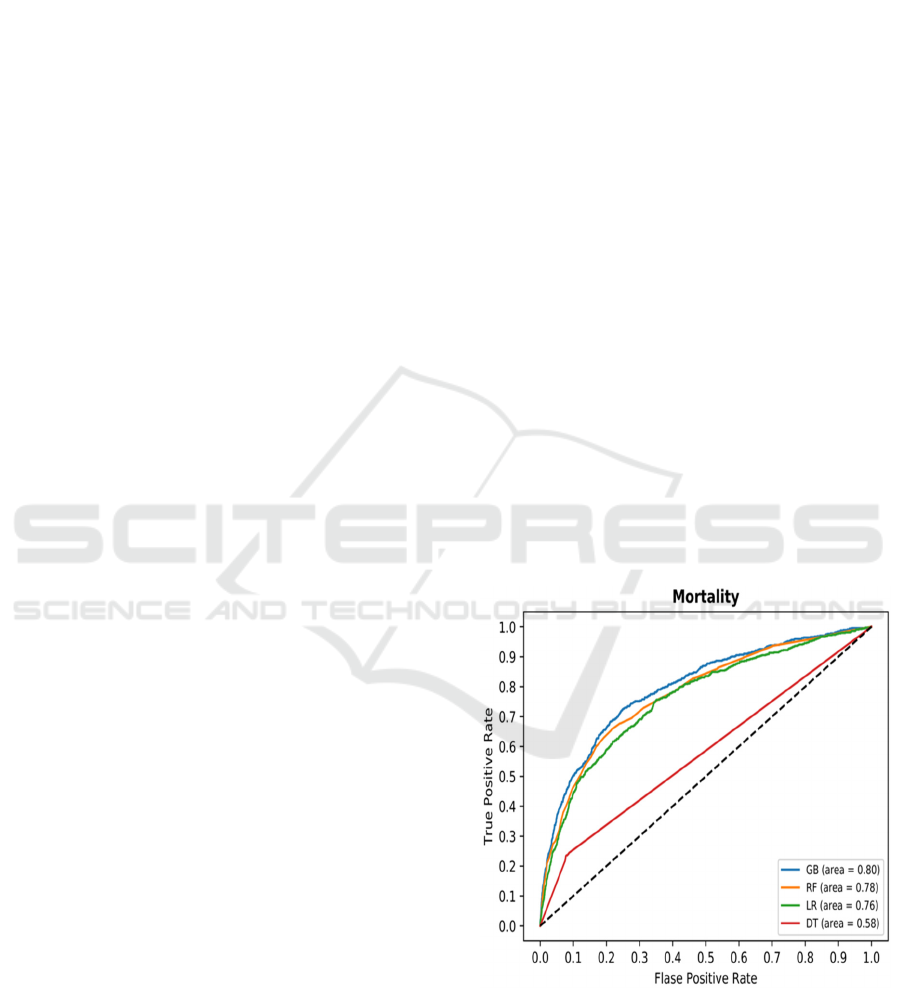
To exemplify these most popular measures, let’s

consider four algorithms applied to prediction of 1-

year mortality (Problem 1): Random Forest

(Breiman, 2001), Gradient Boost (Friedman, 2001;

Friedman, 2002), and Logistic Regression (Hosmer et

al., 2013), and Decision Tree (CART algorithm)

(Breiman et al., 2017; Batra & Agrawal, 2018). ROC

Curves for the four methods are shown in Fig. 2.

Several things are clear from the figure. The curves

for GB, RF and LR models are visually close to each

other with GB slightly dominating the other two. This

is also evident when calculating AROC for the three

models AROC(GB)=0.8, AROC(RF)=0.78, and

AROC(LR)=0.76. The differences are statistically

significant with p<0.05 for t-test over 10-fold cross-

validation. It is also clear that at certain levels of

threshold, GB and RF algorithms perform identically

when the lines overlap.

It is also clear that ROC is ill-defined and AROC

should not be calculated for decision tree-based

models that do not provide probabilistic output but

only the final decision. Literature often presents ROC

curves for decision trees or decision rules with

collected lines as in Fig 2, but this is also misleading,

as only one point exists on the curve. One can argue

that pruned DTs return scores in [0,1] range, but it is

our belief that AROC should not be used for them

either.

Figure 2: Receiver Operator Curves for four algorithms in

predicting 1-year patient mortality.

Similarly, one can compare different models

constructed with different representation spaces as

illustrated in Fig. 3. It shows ROCs for GB-based

models with Binary and Temporal Min-Max

Discussion on Comparing Machine Learning Models for Health Outcome Prediction

713

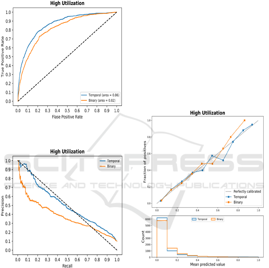
representation. Here, it is clear that the temporal

representation is superior at every possible

classification threshold.

Figure 3: Receiver Operator Curves comparing two

representation spaces in predicting high utilization of

medical services.

Figure 4: Precision-Recall Curves comparing two

representation spaces in predicting high utilization of

medical services.

Some authors argue the benefit of using Precision-

Recall Curves (PRC) and AUCPR instead of AROC.

An example of such curves is shown in Fig. 4 in

predicting high utilization (Problem 2) using GB.

Precision and recall (and F1-score) are calculated

for one specific point on the PRC, which corresponds

to a threshold that is selected by the application.

Interestingly, few works report precision and recall

for classification thresholds other than 0.5, which

makes the direct comparison of models often

impossible based on the two measures. One model

may have higher precision, while other has higher

recall. While F1-score solves the problem by

calculating a single number, it is an

oversimplification. Thus, it is suggested to fix value

of one of the measures and report the other. For

example, precision can be reported at recall of 90%

of both models, or conversely recall can be reported

at precision of 90%.

Calibration (Fig. 5) refers to the property of

models that compare their output probability to the

actual probabilities as defined by frequencies of

positive and negative examples. Numerically,

calibration is quantified with Briar score, that is mean

squared error between scores and probabilities (Flach,

2019).

Figure 5: Calibration plots for two models constructed

using Temporal Min-Max representation and binary

representation.

Finally, it is important to compare models’

performance for specific sub-populations. ROC and

PRCs as well as calibration can be investigated. The

model performance analysis on sup-population has

been popularized with the growing focus on fairness

in Artificial Intelligence (AI). In short, one needs to

check if model accuracy is comparable for sub-

HEALTHINF 2022 - 15th International Conference on Health Informatics

714

populations, especially those representing minorities

and vulnerable populations.

4 OUTPUT COMPARISON

Comparing calibration of models gives good insight

about their outputs and allows for some comparison

at different output levels. However, neither

calibration analysis nor any of the other statistical

methods described in Section 2 provide case-by-case

insights into models’ performance.

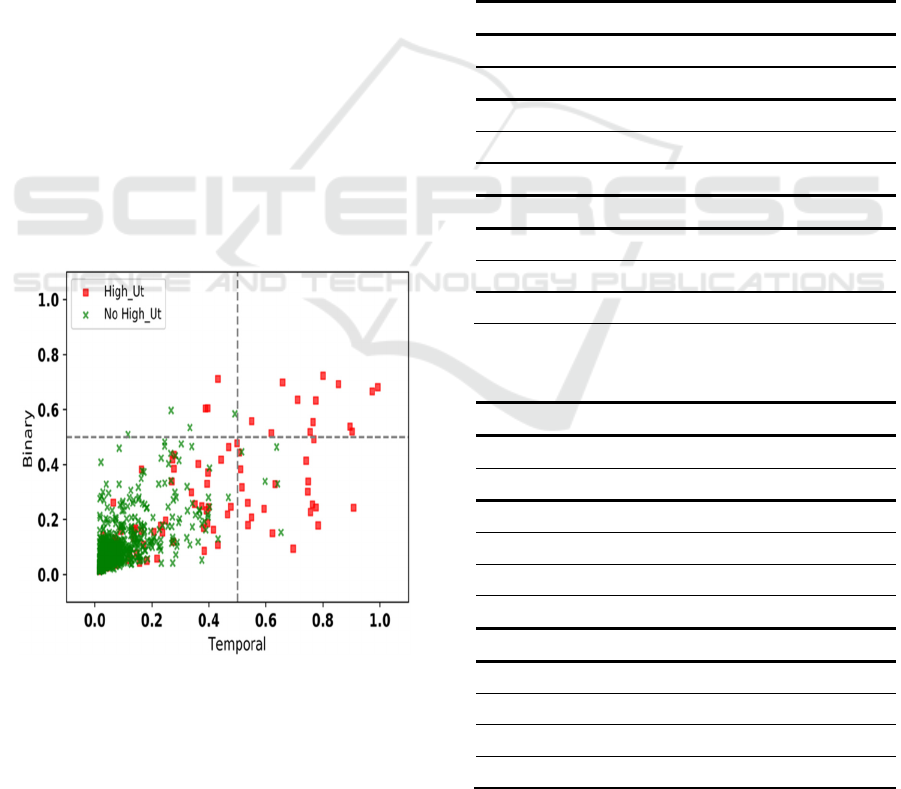
Model Correlation Plots (MCP) allow for visual

case-by-case comparison of model outputs

(Wojtusiak et al., 2017). The MCPs are scatterplots

with axis corresponding to outputs of two models, and

points representing individual cases (i.e., patients) for

which predictions are made. If two models are

identical, all points are located at the diagonal and

M1(x) = M2(x) for every x in dataset (training or

testing). Further, MCPs encode true class by color or

symbol as shown in Fig. 6, which in this case red

points represent high utilizers and green non-high

utilizers, and may include regression lines.

The corresponding aggregated data are presented

in Table 1 for both mortality and high utilization

prediction problems. Wilcoxon signed-rank test was

used to compare the results and significance in

differences is indicated in Table 1.

Figure 6: Model Correlation Plot that compares two

Gradient Boost models based on Binary and Temporal Min-

Max representations in predicting high utilization of

medical services.

When observing values in Fig 6, it is clear that

both sets are nonempty with large number of cases. It

can be also observed that the Temporal Min-Max-

based model tends to produce overall higher scores

for positive test cases. The average output probability

among cases with positive labels was significantly

higher across Temporal Min-Max representation-

based models (also shown in Table 1). Overall, higher

probabilities of positive labels and lower probability

of negative labels in Temporal representation suggest

that this method is generally more likely to correctly

classify both classes. Also, higher recall in Temporal

representation of diagnoses suggests that the method

allows the algorithms to select more positive cases

that are missed in Binary representation method, thus

leading to overall higher recall (Table 2).

Table 1: Comparison of output probability for Temporal

Min-Max (Tem) vs. Binary (Bin) Representations. *

indicates significance (p<0.05).

Problem 1 - Mortality

Positive Label Negative Label

Alg Temp Bin Temp Bin

RF .1859

.1459 .0758

.0765

GB .1883

.1452 .0637

.0674

LR .1579

.1487 .0665

.0673

Problem 2 – High Utilization

RF .3040

.2300 .0879

.0946

GB .3282

.2385 .0748

.0850

LR .2680

.2414 .0817

.0848

Table 2: Comparison of the number correct classified cases

for Temporal Min-Max vs. Binary representations.

Problem 1 - Mortality

Positive Label Negative Label

Alg Temp Bin Temp Bin

RF 143 8 16 75

GB 465 33 67 348

LR 99 28 78 159

DT 980 715 5244 4767

Problem 2 – High Utilization

RF 1115 118 174 417

GB 1443 196 418 811

LR 524 167 240 439

DT 1902 1114 6133 5031

Let’s consider two models 𝑀



and 𝑀



. Let 𝑇𝑆



Discussion on Comparing Machine Learning Models for Health Outcome Prediction

715

a set of examples from the test set TS such that

⋁

𝑀



(𝑥) > 𝑀



(𝑥) + 𝜀

∈



. Similarly, one can

define 𝑇𝑆



⋁

𝑀



(𝑥) < 𝑀



(𝑥) − 𝜀

∈



. The sets

𝑇𝑆



and 𝑇𝑆



define points for which the models

produce higher scores retrospectively. Instead of

counting correct/incorrect cases or calculating

precision and recall, one can compare examples in

sets TS

and TS

. This analysis can be further stratified

by patient demographics and plots constructed

separately for genders, races, age groups, or different

diagnoses. On aggregate, this is equivalent to

calculating Mean Squared Error or Mean Absolute

Error from the 0/1 classification methods.

5 INPUT COMPARISON

Comparing model outputs allows for visually or

statistically inspecting differences between models

on individual cases. However, one needs to

understand if there are any patterns within input

values that correspond to differences in outputs of the

compared models. In other words, are there patterns

in input values that correspond to outputs visualized

in model correlation plots? The patterns can be

described in terms of attributes present in the data or

derived from them.

Let 𝑇𝑆



be a set of positive cases in testing set TS

and 𝑇𝑆



be a set of negative cases in TS. Let’s

consider now four subsets of the testing set.

𝐶𝑃𝑀



={𝑥∈𝑇𝑆



: 𝑀



(𝑥) ≥ 𝜏 ∧ 𝑀



(𝑥) < 𝜏}

𝐶𝑁𝑀



={𝑥∈𝑇𝑆



: 𝑀



(𝑥) < 𝜏 ∧ 𝑀



(𝑥) ≥ 𝜏}

𝑆𝑃𝑀



={𝑥∈𝑇𝑆



: 𝑀



(𝑥) ≥ 𝑀



(𝑥) + 𝜀}

𝑆𝑁𝑀



={𝑥∈𝑇𝑆



:𝑀



(

𝑥

)

<𝑀



(

𝑥

)

−𝜀}

𝐶𝑃𝑀



and 𝐶𝑁𝑀



are respectively positive and

negative cases correctly classified by model 𝑀



but

not 𝑀



. 𝑆𝑃𝑀



and 𝑆𝑁𝑀



are positive and negative

cases better classified by model 𝑀



. These four sets

can be compared in terms of values of input attributes.

The sets 𝐶𝑃𝑀



, 𝐶𝑁𝑀



, 𝑆𝑃𝑀



, and 𝑆𝑃𝑀



are defined

analogously for results superior by model 𝑀



For example, let’s consider again the two

problems of predicting mortality and high utilization

for medical services. Let 𝑀



be model based on

Temporal Min-Max representation and 𝑀



model

based on standard Binary representation. One simple

way to assess patient risk for both problems is a

simple count of underlying medical conditions

(present diagnosis codes). For all cases correctly

classified by one model but incorrectly by another,

what are the counts of present medical conditions.

These numbers are reported in Table 3. Note the

extremely small value 1.1 for Binary representation

in random forest classifier. That number is due to very

small number of cases correctly classified when using

Binary representation and incorrectly with Temporal

Min-Max representation. Similarly, Table 4 presents

values for cases better predicted by one of the models.

Table 3: Comparison of the number of present codes for

Temporal Min-Max vs. Binary representations for correct

predictions.

Problem 1 - Mortality

Positive Label

Negative Label

Alg

Temp

𝐶𝑃𝑀



Bin

𝐶𝑃𝑀



Temp

𝐶𝑁𝑀



Bin

𝐶𝑁𝑀



RF 83.0

1.1 10.5

77.3

GB 77.9 87.0 85.8

78.5

LR 80.0 86.5 84.9

78.8

DT 68.9

65.0 57.8

59.5

Problem 2 – High Utilization

RF 85.3

103.7 101.5

88.9

GB 79.7

97.0 96.8

80.8

LR 85.8

99.7 98.1

85.6

DT 76.9

78.6 63.6

64.0

Table 4: Comparison of the number of present codes for

Temporal Min-Max vs. Binary representations for superior

predictions.

Problem 1 - Mortality

Positive Label

Negative Label

Alg

Temp

𝑆𝑃𝑀



Bin

𝑆𝑃𝑀



Temp

𝑆𝑁𝑀



Bin

𝑆𝑁𝑀



RF 60.68

52.52 46.25

50.13

GB 60.52

52.92 47.71

46.23

LR 57.35 57.08 49.19

45.13

DT 68.46

64.24 56.89

58.49

Problem 2 – High Utilization

RF 71.74

70.50 47.24

50.83

GB 70.70 70.99 49.22

39.08

LR 69.72

72.65 44.79

45.71

DT 76.84

78.54 62.85 63.19

Diving deeper into comparison of the models

constructed with Binary and Temporal Min-Max

representations, it is possible to compare the actual

HEALTHINF 2022 - 15th International Conference on Health Informatics

716

values within cases based on these representations.

Temporal Min-Max representation has more

information than binary representation, and more

specifically the numbers of days. Thus, a reasonable

comparison is one that looks at numbers of days from

diagnoses for cases correctly classified by either of

the models (but not both) as shown in Table 5, or

better predicted by either of the models as shown in

Table 6. The structure of these tables is analogous to

the Tables 3 and 4, but values are average numbers of

days between diagnosis and prediction.

Depending on the actual types of models

constructed and the representation spaces used, one

needs to design appropriate comparisons on input

values. These depend on the nature of data, such as

static or temporal, types of input attributes, numbers

of attributes, and types of models used.

Table 5: Comparison of the average number of days for

Temporal Min-Max vs. Binary representations for correct

predictions.

Problem 1 - Mortality

Positive Label

Negative Label

Alg

Temp

𝐶𝑃𝑀



Bin

𝐶𝑃𝑀



Temp

𝐶𝑁𝑀



Bin

𝐶𝑁𝑀



RF 1259.6* 2599.1 2405.3

1243.4

GB 1353.6 1413.3 1898.0

1380.5

LR 1181.7

1906.9 2608.1

1193.3

DT 1595.1

1680.8 1981.4

1838.6

Problem 2 – High Utilization

RF 1432.5

1913.5 2070.2

1555.0

GB 1468.2

1754.1 1834.7

1525.5

LR 1184.2

2195.7 2362.4

1213.2

DT 1579.9

1669.6 1944.5

1754.2

Another possible way to compare the models is to

construct a model C

M1,M2

that predicts when one

models is significantly better than the other, that is to

classify 𝑆𝑃𝑀



and 𝑆𝑁𝑀



against 𝑆𝑃𝑀



and 𝑆𝑁𝑀



Alternatively, 𝑆𝑃𝑀



against 𝑆𝑃𝑀



can be built if one

is concerned only with positive cases. AROC > 0.5

for such a model indicates a pattern on cases for

which one model dominates the other. Note such a

model does not tell us if either of the models 𝑀



𝑀



are correct, but rather which is more likely to

produce a better result for a given case. Typically, one

should prefer CM1,M2 to be an easy to interpret

model such as logistic regression or decision tree so

that conclusions can be drawn from the discovered

patterns.

Table 6: Comparison of the average number of days for

Temporal Min-Max vs. Binary representations for superior

predictions.

Problem 1 - Mortality

Positive Label

Negative Label

Alg

Temp

𝑆𝑃𝑀



Bin

𝑆𝑃𝑀



Temp

𝑆𝑁𝑀



Bin

𝑆𝑁𝑀



RF 1641.26

1771.76 1920.35

1816.88

GB 1549.92

1896.64 2004.06

1699.10

LR 1510.49

1933.96 2103.39

1643.55

DT 1600.81

1682.96 1977.14

1842.69

Problem 2 – High Utilization

RF 1538.88

1795.15 2048.76

1644.65

GB 1497.31

1833.94 2055.30

1587.85

LR 1338.79

2082.75 2188.95

1459.63

DT 1579.53

1669.15 1942.51

1755.21

6 CONCLUSIONS

Model comparison is not a trivial task. Through

comparisons, one can select the best model, but also

gain useful insight into why specific models perform

differently than others. It is clear that comparing

models based on accuracy alone is not sufficient.

This position paper was not intended to present

the best models or results for specific problems, nor

to argue for the use of specific modeling methods.

The two examples were used only for informative

purposes and could be replaced with any other cases.

The paper did also not mean to provide a full set of

metrics and tasks to be performed in comparing

models. Selection of the specific metrics should be

done carefully to gain maximum insights into the

application area. Instead, this paper was intended to

contribute to an ongoing discussion on model

evaluation and comparison. With ML field being

dominated with statistical methods, researchers often

assume that statistical model evaluation and

comparison are sufficient. This cannot be further

from the truth, especially in the medical or health care

fields in which every “test case” is a patient whose

treatments and potentially life-altering decisions may

be made based on predictions.

While presented in a different order, the presented

methodology fits into a general framework used by

Discussion on Comparing Machine Learning Models for Health Outcome Prediction

717

the authors in which models are described by their

inputs, models themselves and their outputs. The

framework can be used to study model performance,

explainability, fairness, and other factors that may

ultimately lead to end users’ trust and model

adoption. It emphasizes the concept of machine

learning that makes sense, in which the application of

machine learning results in correctly constructed and

evaluated models for which inputs mimic measurable

real-world characteristics or modeled objects, and

outputs directly correspond to outcomes of interest.

REFERENCES

Baldi, P., Brunak, S., Chauvin, Y., Andersen, C. A., & Nielsen,

H. (2000). Assessing the accuracy of prediction algorithms

for classification: an overview. Bioinformatics, 16(5), 412-

424.

Batra, M., & Agrawal, R. (2018). Comparative analysis of

decision tree algorithms. In Nature inspired computing (pp.

31-36). Springer, Singapore.

Beaulieu-Jones, B. K., Yuan, W., Brat, G. A., Beam, A. L.,

Weber, G., Ruffin, M., & Kohane, I. S. (2021). Machine

learning for patient risk stratification: standing on, or looking

over, the shoulders of clinicians?. NPJ digital medicine, 4(1),

1-6.

Boyd, K., Eng, K. H., & Page, C. D. (2013, September). Area

under the precision-recall curve: point estimates and

confidence intervals. In Joint European conference on

machine learning and knowledge discovery in databases (pp.

451-466). Springer, Berlin, Heidelberg.

Breiman, L. (2001). Random forests. Machine learning, 45(1), 5-

32.

Breiman, L., Friedman, J. H., Olshen, R. A., & Stone, C. J. (2017).

Classification and regression trees. Routledge.

Castellazzi, G., Cuzzoni, M. G., Cotta Ramusino, M., Martinelli,

D., Denaro, F., Ricciardi, A., ... & Gandini Wheeler-

Kingshott, C. A. (2020). A machine learning approach for the

differential diagnosis of Alzheimer and Vascular Dementia

Fed by MRI selected features. Frontiers in

neuroinformatics, 14, 25.

Fawcett, T. (2006). An introduction to ROC analysis. Pattern

recognition letters, 27(8), 861-874.

Flach, P. (2019, July). Performance evaluation in machine

learning: the good, the bad, the ugly, and the way forward. In

Proceedings of the AAAI Conference on Artificial

Intelligence (Vol. 33, No. 01, pp. 9808-9814).

Friedman, J. H. (2001). Greedy function approximation: a

gradient boosting machine. Annals of statistics, 1189-1232.

Friedman, J. H. (2002). Stochastic gradient boosting.

Computational statistics & data analysis, 38(4), 367-378.

Goutte, C., & Gaussier, E. (2005, March). A probabilistic

interpretation of precision, recall and F-score, with

implication for evaluation. In European conference on

information retrieval (pp. 345-359). Springer, Berlin,

Heidelberg.

Hanley, J. A., & McNeil, B. J. (1982). The meaning and use of

the area under a receiver operating characteristic (ROC)

curve. Radiology, 143(1), 29-36.

Hosmer Jr, D. W., Lemeshow, S., & Sturdivant, R. X. (2013).

Applied logistic regression (Vol. 398). John Wiley & Sons.

McDermott, M. B., Wang, S., Marinsek, N., Ranganath, R.,

Foschini, L., & Ghassemi, M. (2021). Reproducibility in

machine learning for health research: Still a ways to go.

Science Translational Medicine, 13(586).

McHugh, M. L. (2012). Interrater reliability: the kappa statistic.

Biochemia medica, 22(3), 276-282.

Mehrabi, N., Morstatter, F., Saxena, N., Lerman, K., & Galstyan,

A. (2021). A survey on bias and fairness in machine learning.

ACM Computing Surveys (CSUR), 54(6), 1-35.

Lee, E. A., & Sangiovanni-Vincentelli, A. (1998). A framework

for comparing models of computation. IEEE Transactions on

computer-aided design of integrated circuits and systems,

17(12), 1217-1229.

Powers, D. M. (2020). Evaluation: from precision, recall and F-

measure to ROC, informedness, markedness and correlation.

arXiv preprint arXiv:2010.16061.

Rahane, W., Dalvi, H., Magar, Y., Kalane, A., & Jondhale, S.

(2018, March). Lung cancer detection using image

processing and machine learning healthcare. In 2018

International Conference on Current Trends towards

Converging Technologies (ICCTCT) (pp. 1-5). IEEE.

Saha, P., Sadi, M. S., & Islam, M. M. (2021). EMCNet:

Automated COVID-19 diagnosis from X-ray images using

convolutional neural network and ensemble of machine

learning classifiers. Informatics in medicine unlocked, 22,

100505.

Tseng, Y. J., Wang, H. Y., Lin, T. W., Lu, J. J., Hsieh, C. H., &

Liao, C. T. (2020). Development of a machine learning

model for survival risk stratification of patients with advanced

oral cancer. JAMA network open, 3(8), e2011768-e2011768.

Vaccaro, M. G., Sarica, A., Quattrone, A., Chiriaco, C., Salsone,

M., Morelli, M., & Quattrone, A. (2021).

Neuropsychological assessment could distinguish among

different clinical phenotypes of progressive supranuclear

palsy: A Machine Learning approach. Journal of

Neuropsychology, 15(3), 301-318.

Wang, Q., Ma, Y., Zhao, K., & Tian, Y. (2020). A comprehensive

survey of loss functions in machine learning. Annals of Data

Science, 1-26.

Wojtusiak, J., Elashkar, E., & Nia, R. M. (2017, February). C-

Lace: Computational Model to Predict 30-Day Post-

Hospitalization Mortality. HEALTHINF 2017 (pp. 169-177).

Wojtusiak J. Reproducibility, Transparency and Evaluation of

Machine Learning in Health Applications. HEALTHINF

2021 (pp. 685-692).

Wojtusiak, J., Asadzaehzanjani, N., Levy, C., Alemi, F., &

Williams, A. E. (2021). Online Decision Support Tool that

Explains Temporal Prediction of Activities of Daily Living

(ADL). HEALTHINF 2021 (pp. 629-636).

Wojtusiak, J., Asadzadehzanjani, N., Levy, C., Alemi, F., &

Williams, A. E. (2021). Computational Barthel Index: an

automated tool for assessing and predicting activities of daily

living among nursing home patients. BMC medical

informatics and decision making, 21(1), 1-15.

HEALTHINF 2022 - 15th International Conference on Health Informatics

718