Transfer Learning via Test-time Neural Networks Aggregation

Bruno Casella

1,2 a

, Alessio Barbaro Chisari

3,4 b

, Sebastiano Battiato

4 c

and Mario Valerio Giuffrida

5 d

Department of Computer Science, University of Torino, Torino, Italy

Department of Economics and Business, University of Catania, Catania, Italy

Department of Civil Engineering and Architecture, University of Catania, Catania, Italy

Department of Mathematics and Computer Science, University of Catania, Catania, Italy

School of Computing, Edinburgh Napier University, Edinburgh, U.K.

Keywords:

Parameter Aggregation, Transfer Learning, Selective Forgetting.

Abstract:

It has been demonstrated that deep neural networks outperform traditional machine learning. However, deep

networks lack generalisability, that is, they will not perform as good as in a new (testing) set drawn from a

different distribution due to the domain shift. In order to tackle this known issue, several transfer learning

approaches have been proposed, where the knowledge of a trained model is transferred into another to im-

prove performance with different data. However, most of these approaches require additional training steps,

or they suffer from catastrophic forgetting that occurs when a trained model has overwritten previously learnt

knowledge. We address both problems with a novel transfer learning approach that uses network aggregation.

We train dataset-speciﬁc networks together with an aggregation network in a uniﬁed framework. The loss

function includes two main components: a task-speciﬁc loss (such as cross-entropy) and an aggregation loss.

The proposed aggregation loss allows our model to learn how trained deep network parameters can be aggre-

gated with an aggregation operator. We demonstrate that the proposed approach learns model aggregation at

test time without any further training step, reducing the burden of transfer learning to a simple arithmetical

operation. The proposed approach achieves comparable performance w.r.t. the baseline. Besides, if the aggre-

gation operator has an inverse, we will show that our model also inherently allows for selective forgetting, i.e.,

the aggregated model can forget one of the datasets it was trained on, retaining information on the others.

1 INTRODUCTION

Deep Learning (DL) has demonstrated superior per-

formance than traditional ML methods in a variety of

tasks. This is due to being able to extract discrimi-

native features from the data for the task at hand via

end-to-end training. Such discriminative features are

suitable for the dataset the network was trained on.

However, a deep network will not perform as good

as in a different dataset due to the domain shift (or

dataset bias) (Zhao et al., 2020).

A way to address the domain shift is via Trans-

fer Learning (TL), where the information learnt by

a trained network is (re)used in another context.

https://orcid.org/0000-0002-9513-6087

https://orcid.org/0000-0002-7831-382X

https://orcid.org/0000-0001-6127-2470

https://orcid.org/0000-0002-5232-677X

Several approaches to transfer learning have been

proposed in literature, such as sample reweighting

(Sch

olkopf et al., 2007), feature distributions minimi-

sation (Tzeng et al., 2017; Litrico et al., 2021), dis-

tillation (Hinton et al., 2015), and so on (for a recent

survey on TL, please read (Zhuang et al., 2021)).

However, transfer learning techniques may be af-

fected by catastrophic forgetting (Goodfellow et al.,

2013), where a network forgets the information learnt

from a previous task when transferred to a new one.

Furthermore, generally, transfer learning requires fur-

ther training steps to accommodate for new data, even

though the learnt task remains unchanged.

The beneﬁt of transfer learning has been demon-

strated extensively in the last years (Weiss et al.,

2016), even in distributed training scenario (Chen

et al., 2020). In this context, a central model is

trained on several datasets that have never directly

seen, as they are located in different machines (feder-

642

Casella, B., Chisari, A., Battiato, S. and Giuffrida, M.

Transfer Learning via Test-time Neural Networks Aggregation.

DOI: 10.5220/0010907900003124

In Proceedings of the 17th International Joint Conference on Computer Vision, Imaging and Computer Graphics Theory and Applications (VISIGRAPP 2022) - Volume 5: VISAPP, pages

642-649

ISBN: 978-989-758-555-5; ISSN: 2184-4321

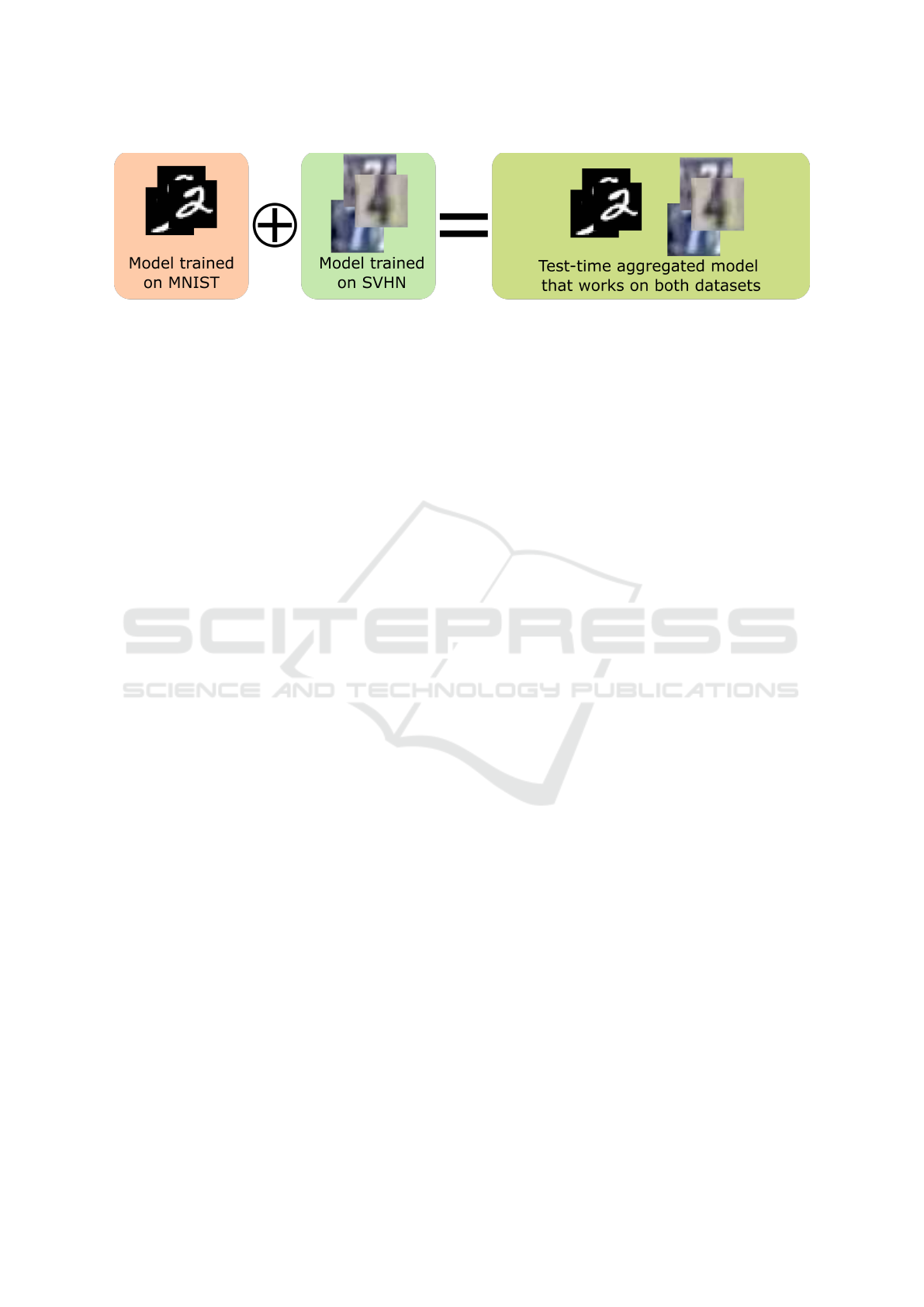
Figure 1: Pictorial representation of the proposed method that performs test-time neural network aggregation.

ated learning). However, this training paradigm raised

another question: what if one (or more) datasets used

to train the centrally trained model needs to be re-

moved? Machine unlearning (Golatkar et al., 2021) is

studied for several reasons, especially when sensible

data are used (e.g., medical imaging). However, it is

generally hard to selectively scrub the parameters of a

model such that it cannot perform well on a portion of

the dataset, whilst it retains comparable performance

as before on the rest of the dataset.

In this paper, we propose a new proof-of-concept

technique to TL that inherently allows for selec-

tive forgetting by aggregating the network parameters

without any further training. This can be applied to

different datasets, assuming they all share the same

task. Our approach is represented in Figure 1 and

works as follows: we train a VGG-like (Simonyan

and Zisserman, 2015) deep neural network for each

dataset – we will refer to these networks as N

, for

i = 1, ...,n, with n being the number of datasets. In

addition, a VGG-like network – named N

∗

– is also

trained taking all the datasets as inputs. All the net-

works are trained end-to-end with a aggregation regu-

lariser, ensuring that the weights learnt by N

∗

are ob-

tained as an aggregation for all the other networks N

This training paradigm will ensure that the networks

also learn how to be aggregated. Furthermore, re-

quiring that the aggregation function is invertible, our

model inherently allows for selective forgetting. In

our experiments, we set n = 2 datasets, and we used

the sum of weights as network aggregation function

(which can easily be inverted with subtraction), which

is applied to only the parameters of the feature extrac-

tors. All the networks trained within this end-to-end

framework (including N

∗

) share the same classiﬁer.

Experimental results show that test-time network ag-

gregation is possible, outperforming the baseline.

The key contributions of our approach can be sum-

marised as follows:

1. we propose the aggregation regulariser during

training;

2. network aggregation is achieved at test time (no

further training is required);

3. our transfer learning technique does not suffer

from catastrophic forgetting;

4. our approach can also be used for selective for-

getting (assuming networks are aggregated via an

invertible function).

The rest of the paper is organised as follows. In

Section 2, we discuss the recent related works. Sec-

tion 3 outlines our proposed approach. In Section 4,

experimental results are shown and discussed. Fi-

nally, Section 5 concludes the paper.

2 RELATED WORK

The aggregation of network parameters is a form of

transfer learning. Typically, TL generally addresses

a better initial and steeper growth performance (Tom-

masi et al., 2010) by reuse of the convolutional ﬁlter

parameters of CNNs. For example, ﬁne-tuning is the

simplest way to achieve transfer learning: a model,

pre-trained on a dataset, e.g. ImageNet (Deng et al.,

2009), is used as starting point for other datasets and

tasks (Reyes et al., 2015). Although intuitive and easy

to do, ﬁne-tuning typically underperforms wrt other

transfer learning approaches (Shu et al., 2021; Han

et al., 2021). More sophisticated methods have been

proposed (Oquab et al., 2014), but several of them

suffer from negative transfer (Rosenstein et al., 2005;

Pan and Yang, 2010; Torrey and Shavlik, 2010; Wang

et al., 2018; Zhuang et al., 2021): the process of trans-

ferring knowledge is harmful because the knowledge

is not transferable across all the domains (in particular

when the source and target datasets are not related).

Another issue affecting transfer learning ap-

proaches is catastrophic forgetting, where new

knowledge permanently replaces information learnt

from previous tasks (Goodfellow et al., 2013). In

fact, several approaches to TL, such as Batch Spectral

Shrinkage (Chen et al., 2019), attempts to solve such

an issue. However, these approaches still rely on a

training procedure to adapt to a new dataset (or task).

However, we asked ourselves the following question:

Transfer Learning via Test-time Neural Networks Aggregation

643

is it possible achieving TL without catastrophic for-

getting at test time? We achieve that by aggregating

the weights of trained networks together.

The idea of aggregating the parameters of deep

neural networks is not new in the literature. A frame-

work that aggregates knowledge from multiple mod-

els is the Transfer-Incremental Mode Matching (T-

IMM) (Geyer et al., 2019), which enables for adap-

tive merging of models. It is a re-interpretation of

IMM (Lee et al., 2017), a work in the context of life-

long learning aiming at the sequential aggregation of

models retaining good performance on all the prior

tasks, rather than on transfer learning. T-IMM be-

longs to the ﬁeld of incremental learning, a subtly dif-

ferent area concerning lifelong learning, in which the

parameters of the i-th model are used as initialisation

for model i + 1. More recently, Zoo-Tuning was pro-

posed to adaptively aggregate multiple trained models

(Shu et al., 2021). To achieve network aggregation,

the authors proposed the AdaAgg layer. However, this

approach assumes that models are already pre-trained

before being aggregated (involving a two-step learn-

ing). In our work, models are randomly initialised and

then trained once end-to-end and simultaneously.

Lifelong (or continual) learning describes the sce-

nario in which new tasks arrive sequentially and

should be incorporated into the current model, re-

taining previous knowledge (Parisi et al., 2019). Ap-

proaches to lifelong learning are mainly aimed to mit-

igate catastrophic forgetting (Rao et al., 2019; Rama-

puram et al., 2020; Ye and Bors, 2020). According to

Parisi et al. (2019), there are three main approaches

to lifelong learning: (i) retraining with regularisation;

(ii) network expansion; (iii) selective network retrain-

ing and expansion. In the ﬁrst case, neural networks

are retrained with constraints to prevent forgetting.

Network expansion approaches perform architectural

changes (e.g., adding neurons) to the network to add

novel information. The last approaches update only a

subset of neurons and allow expansion (if necessary).

Our proposed method loosely follows the paradigm

of regularisation approaches with an important differ-

ence: no retraining of the architecture is performed

neither transfer learning nor selective forgetting.

Our approach to network aggregation inherently

allows network decomposition for selective forget-

ting. Recently, several related works have focused on

machine unlearning (Golatkar et al., 2020; Golatkar

et al., 2021). Overall, these approaches assume that

the portion of the dataset that the model should un-

learn is given to a scrub function that aims to remove

the information learnt from the dataset to be forgot-

ten, impacting (although minimally) the performance

of the scrubbed model on the rest of the dataset. Our

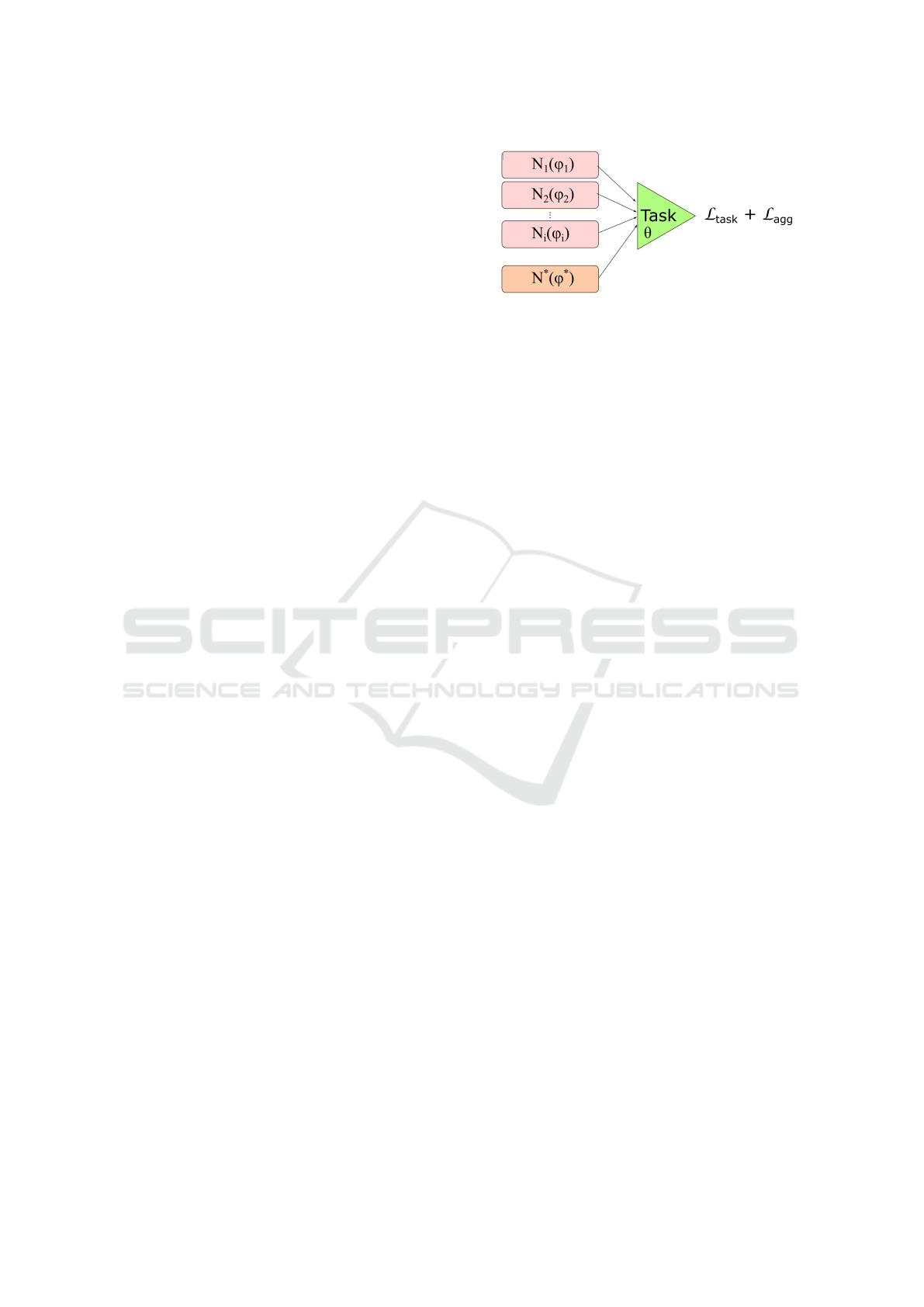
Figure 2: Graphical representation of the proposed method.

Each network N

is parametrised by a set of weights ϕ

. The

aggregated network N

∗

is parametrised by ϕ

∗

. There is no

weight sharing between these networks. However, all the

networks share the same task network (i.e., a classiﬁer). The

total objective function is given as a combination two loss

functions: (i) task loss (i.e., cross-entropy); (ii) aggregation

loss (see Section 3.3).

approach is different: we do not require data to be

provided for selective forgetting. Instead, the aggre-

gated model trained on two (or more) datasets can be

changed by applying the inverse of the aggregation

function (in our case, a simple subtraction).

3 PROPOSED METHOD

Figure 2 displays the proposed approach: the general

idea is to aggregate the weights of two different neu-

ral networks trained on two different datasets (shar-

ing the same underlying task). The ultimate goal is to

obtain n individual networks N

such that their com-

position N

⊕ N

⊕ . .. ⊕ N

≈ N

∗

(note that the oper-

ator ⊕ refers to a generic network aggregation oper-

ator, which details will be provided in Section 3.3).

Below, we will refer to an individual network N

dataset-speciﬁc network, whereas N

∗

will be referred

to as aggregated network. As anticipated in Section 1,

all these networks used as feature extractors share the

same task network.

3.1 Task Network

As shown in Figure 2, the task network is shared

across the aggregated and dataset-speciﬁc networks.

This network is parametrised by the set of weights θ:

the output provided by all of the N

and N

∗

is used as

input of the task network, and its output is the predic-

tion (i.e., softmax activation in case of classiﬁcation).

The task network is trained with a task-speciﬁc

loss function as L

(z,y; w), that takes the training data

z (in form of representation) and target variables y as

inputs, and it is parametrised by a set of weights w

(that includes θ and the parameters of the feature ex-

tractors). We used cross-entropy loss for L

in this

VISAPP 2022 - 17th International Conference on Computer Vision Theory and Applications

644

paper. For other tasks (i.e., regression), a different

loss function may be used (e.g., mean squared error).

3.2 Dataset-speciﬁc Network

Each dataset-speciﬁc network N

acts as a feature ex-

tractor for the dataset it is trained on. We opted to

use a VGG-like network (Simonyan and Zisserman,

2015) in our experiments. In particular, following the

same architectural tweaks as others (Loh et al., 2021),

we used a VGG-16 network with Group Normalisa-

tion (Wu and He, 2018).

Each network N

is parametrised by the set of

weights ϕ

that is trained via standard supervised

learning. In fact, each N

is trained with a different

label dataset; all of those datasets maintain the same

underlying task. This means that each dataset D

con-

tains a set of input data X

, such that x

(i)

∈ X

, and a

set of target values Y

, such that y

(i)

∈ A (the set A

is a generic set deﬁned by the task, i.e. if the task is

classiﬁcation, A will contain all the possible classes).

For each of these networks, a speciﬁc loss func-

tion is used during training:



(i)

;φ

∪ θ



= L



(i)



(i)

;φ

∪ θ



(1)

3.3 Aggregated Network

The aggregated network is similar to the dataset-

speciﬁc networks: it shares the same architecture but

not the weights. In fact, this network is parametrised

by the set of weights φ

∗

The aggregated network is trained such that its

weights can be expressed as a sum of the dataset-

speciﬁc networks. To achieve this, we proposed the

aggregation regulariser. Each network N

is made

of L

layers, and each layer ` is parametrised by

some weights W

∈ϕ

Similarly, the aggregated net-

work N

∗

includes several layers L, each of those is

parametrised by W

. However, it is important to em-

phasise that all the feature extractors share the same

architecture, that is, L = L

= L

= .. . = L

During training, we want that:

= W

⊕ W

⊕ . . . ⊕ W

, (2)

We also tried either Batch Normalisation (Ioffe and

Szegedy, 2015) or no normalisation with no success.

Some types of layers, for example, convolutional lay-

ers, can be parametrised by multiple weights, such as ker-

nels and bias. For the sake of clarity, we incorporate these

weights within W

i.e., the weights at layer ` in the aggregated network

should be equal to the aggregation of the correspond-

ing layer weights in the dataset-speciﬁc networks.

We reformulate this constrain as a regulariser during

training. Assuming that  is the inverse operator of

⊕, the aggregation regulariser is then expressed as:

agg

(Φ) =

∑

`=1



⊕ W

⊕ . . . ⊕ W

, (3)

where Φ = φ

∗

∪ (

i=1

) is the set of all the weights

in all the feature extractors.

Although the networks

learn a non-linear mapping w.r.t the task, the aggrega-

tion regulariser in Equation (3) learns the weights Φ

such that the network aggregation can be performed

with a linear operation (assuming that ⊕ is linear).

The aggregated network takes all the input data

that are used for each dataset-speciﬁc network D =

i=1

and it is trained in a supervised manner w.r.t.

the task L

as follows:

∗

(x, y;φ

∗

∪ θ) = L

∗

(x),y, φ

∗

∪ θ), (4)

where (x,y) ∈ D, i.e. inputs and labels are taken from

all the datasets used to train the dataset-speciﬁc net-

works.

3.4 Objective Function

As shown in Figure 2, the objective functions used to

train our model is the following:

J(x, y;Θ) = L

task

+ L

agg

, (5)

where Θ = Φ ∪ θ is the set of all the parameters in

the network. the loss function L

task

is given as the

sum of all the task-speciﬁc loss functions expressed

in Equation (1) and Equation (4):

task

(x, y;Θ) = L

∗

(x, y;φ

∗

∪ θ)

∑

i=1



(i)

;φ

∪ θ



After training, there is no guarantee that the regu-

lariser in Equation (3) ensures that Equation (2) is sat-

isﬁed. However, the optimisation of Equation (5) will

make sure that W

≈ W

⊕ W

⊕ . . . ⊕ W

. Hence, we

can retrieve N

∗

by aggregating all the weights trained

for each dataset-speciﬁc network N

– we will refer to

this model as

∗

, such that

∗

≈ N

∗

Similarly as in (Geyer et al., 2019), we only aggregate

weights of convolutional layers.

Transfer Learning via Test-time Neural Networks Aggregation

645

We can selectively forget one of the datasets from

∗

by applying a simple arithmetic operation. As-

suming that we wanted to remove the k-th dataset, we

can perform the operation

∗

 N

, without any fur-

ther training (or adaptation) steps.

3.5 Implementation Details

We set the number of datasets (and thus the number

of dataset-speciﬁc networks) to n = 2. This allowed

us to demonstrate whether our approach works and

to set a baseline. We set the number of groups for

Group Normalisation to 32. We used as aggregation

operator the sum for the following reasons: (i) it has

an inverse – the subtraction; (ii) it is differentiable.

We set as task-speciﬁc loss function the cross-entropy

loss as we train the whole network for a classiﬁcation

task. Stochastic Gradient Descent (SGD) was used as

optimiser for training with a learning rate η = 0.01.

The baseline was trained for 20 epochs, while train-

ing of our proposed method lasted 200 epochs. We

implemented our approach in PyTorch (Paszke et al.,

2019) on Google Colaboratory.

4 EXPERIMENTAL RESULTS

Dataset. we used MNIST (LeCun et al., 2010) as

and SVHN format 2 (Netzer et al., 2011) as

. MNIST contains 60, 000 binary images of size

28 × 28 for training and 10,000 images for testing.

SVHN contains 73, 257 colour images of size 32× 32

for training and 26,032 for testing. We chose these

two datasets for the following reasons: (i) they are

designed for the same classiﬁcation (10-class) task;

(ii) data are drawn from different distributions.

Preprocessing. In order to use the same architecture

for both datasets, MNIST images were rescaled to

32 × 32. We converted the SVHN images in binary

(grayscale). As for data augmentation, we performed

random horizontal ﬂips with a probability of 50%.

Baseline. We compared our method with a standard

VGG-16 network with Batch Normalisation (Ioffe

and Szegedy, 2015). We ran the following baseline

experimentation:

1. trained it only on MNIST – following the nota-

tion adopted in this paper, we called this trained

network N

;

2. trained it only on SVHN – named N

;

3. trained it on both (N

∗

);

4. The weights trained on N

and N

were taken to

perform N

⊕ N

at test time.

Experimental results are shown in Table 1.

Table 1: Testing performance of the proposed method com-

pared to the baseline performance. D

indicates MNIST;

indicates SVHN. The models obtained via aggregation

(i.e., N

⊕ N

) are obtained at test time by aggregating the

weights of the networks.

Trained on Tested on

∪ D

Baseline

 – 99.04% 8.67% 33.75%

–  57.63% 90.29% 80.78%

∗

  98.73% 90.58% 92.85%

⊕ N

  9.75% 7.59% 8.19%

Proposed Method

 – 98.90% 41.45% 57.35%

–  45.30% 92.41% 79.31%

∗

  98.40% 86.47% 89.77%

⊕ N

  96.41% 68.03% 75.88%

4.1 Discussion

Our purpose is to demonstrate that the performance

of our aggregated network N

⊕ N

is better than the

baseline. Overall, our method achieves comparable

performance with the baseline for individual tasks

(i.e., N

and N

). However, there is a slight loss in per-

formance in N

∗

, that is, the network trained on both

MNIST and SVHN, with our method. The baseline

achieves approx. 92% accuracy, whereas N

∗

trained

with our method achieves approx. 89%.

Although this minor performance reduction, our

method achieves high performance with test-time

weight aggregation. After N

and N

are trained with

the baseline and our method, weights are aggregated

by applying the ⊕ operator. Table 1 clearly shows

that our training procedure outperforms the baseline

(8% vs 75% testing accuracy). This demonstrates that

a traditional training of two networks cannot be ag-

gregated, leading to catastrophic forgetting on both

datasets. Our training approach with Equation (3) en-

ables the networks to explicitly learn an aggregation

operation that can be reproduced at test time.

Ideally, the performance of N

⊕ N

should be as

close as possible to N

∗

. As shown in the last two lines

of Table 1, there is an approximate loss of 14% ac-

curacy. We hypothesise several reasons for this gap

in accuracy: (i) our method may require more train-

ing time; (ii) Group Normalisation may be having an

impact at test time (as speciﬁed in Section 3.3, we

only aggregate the weights of convolutional layers);

(iii) use of Weight Standardisation (WS) can improve

performance (Qiao et al., 2019; Loh et al., 2021).

In relation to training time, we plot the training

and validation accuracies and losses of our method

VISAPP 2022 - 17th International Conference on Computer Vision Theory and Applications

646

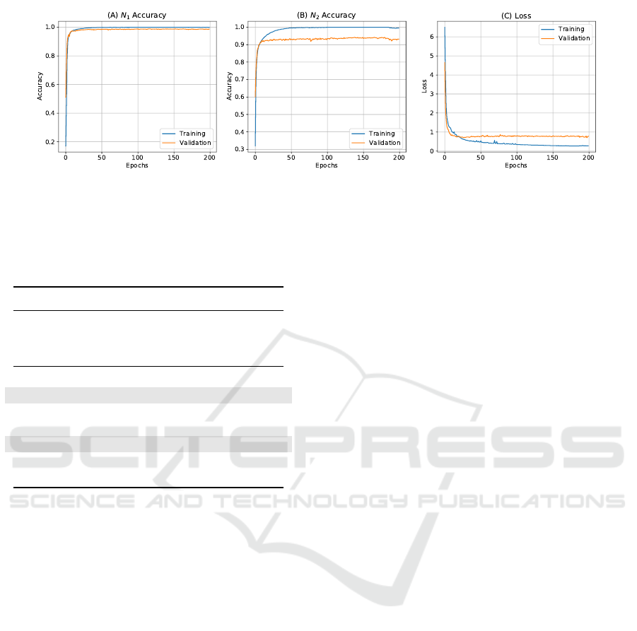
Figure 3: Training and validation accuracies and losses of our proposed method. (A) N

training and validation accuracies;

(B) N

training and validation accuracies; (C) Total training and validation loss.

Table 2: Commutativity and Selective forgetting testing re-

sults. The training is performed in both D

and D

. The

two datasets are the same as in Table 1. Highlighted rows

are copied from Table 1 to ease comparison.

∪ D

Commutativity

⊕ N

96.41% 68.03% 75.88%

⊕ N

96.41% 68.03% 75.88%

Selective forgetting

98.90% 41.45% 57.35%

⊕ N

)  N

98.55% 47.90% 61.92%

⊕ N

)  N

98.55% 47.90% 61.92%

45.30% 92.41% 79.31%

⊕ N

)  N

34.67% 90.88% 75.28%

⊕ N

)  N

34.67% 90.88% 75.28%

in Figure 3. Overall, it can be noted that 50 epochs

should be enough to accommodate for both datasets.

However, we found experimentally that more train-

ing time results in higher performances in our aggre-

gated model. We hypothesise that the optimisation of

Equation (3) could require more time to learn better

aggregable models. In relation to Weight Standardi-

sation, we posit that an increase in performance may

be achievable if the aggregation function is changed

to the mean instead of the sum. Otherwise, the aggre-

gated weights will no longer be zero-centred.

4.2 Commutativity

Here, we want to demonstrate whether our method

is commutative: does the performance of N

⊕ N

match the performance of N

⊕ N

? Theoretically,

commutativity should be strictly related to the ⊕ op-

erator. However, this is not exactly guaranteed in

our framework because we only aggregate the con-

volution weights in the networks N

(see Section 3.3).

Group Normalisation layers also include learnable pa-

rameters that are not included during network aggre-

gation. To conﬁrm whether our method is commu-

tative, we also performed the operation N

⊕ N

and

results are reported in Table 2. It can be seen that the

performances in both scenarios are the same. Hence,

we can conclude that our approach is commutative.

4.3 Selective Forgetting

For the same reasons as in Section 4.2, we also exper-

imentally show whether selective forgetting is possi-

ble with our method. Because of Group Normalisa-

tion layers, (N

⊕ N

) N

≈ N

, i.e., by removing the

contribution of N

, we do not exactly obtain N

(and

vice versa). Therefore, we asked the following ques-

tion: does the network obtained by (N

⊕ N

)  N

perform as good as N

? Table 2 shows the experi-

mental results of selective forgetting.

Forgetting SVHN. We removed the weights of N

from the aggregated networks (we considered N

⊕ N

and N

⊕ N

as aggregated networks), and we pro-

vided the SVHN testing set to this new network.

The testing accuracy is 47.90%, against the 41.45%

of N

. Therefore, the resulting network does forget

about SVHN, although not completely (there is ap-

prox +6% increase of performance).

Forgetting MNIST. A similar experiment was per-

formed by removing the weights of N

from the ag-

gregated networks. Differently than before, the test-

ing accuracy of the resulting network is 34.67%, com-

pared with 45.30%. This experimentally demon-

strates that our method has completely forgotten the

information learnt from the MNIST dataset.

Retained Information. In the two previous exper-

iments, it was shown that the resulting network had

forgotten information from either of the two datasets.

However, we must check whether the network can

still perform well in the other dataset. Overall, the

performance on MNIST dataset is very similar (from

98.90% to 98.55%), whereas in the case of SVHN

there is approx 2% loss of performance (from 92.41%

to 90.88%) – although the overall testing error is

above 90%. This also demonstrates that the proposed

Transfer Learning via Test-time Neural Networks Aggregation

647

method retains information from both tasks with a

loss in performance up to 2%.

5 CONCLUSIONS

In this paper, we proposed a novel and simple proof-

of-concept transfer learning approach that inherently

allows for selective forgetting. Our training method

enables for network aggregation at test time, i.e. the

weights of two networks (trained on two different

datasets) are aggregated together, such that the result-

ing network can work on both datasets without any

further training/adaptation step.

We achieve that by introducing an aggregation

regulariser, that enables the networks to also learn

the aggregation operation in an end-to-end training

framework. We used the sum as aggregation operator,

as it is invertible and differentiable. VGG-like archi-

tectures were used as feature extractors, using Group

Normalisation in lieu of Batch Normalisation.

Our experimental results demonstrated that the

proposed approach allows for test-time transfer learn-

ing without any further training steps. Furthermore,

we showed that our training procedure is commuta-

tive: the aggregated network N

⊕ N

obtains the same

performance of N

⊕ N

. Moreover, we demonstrated

that our method allows for selective forgetting (at the

cost of up to 2% testing performance).

The proposed method has some limitations: (i) it

requires that all the networks involved in the training

share the same architecture; (ii) the selective forget-

ting does not allow to forget a subset of the dataset;

(iii) we evaluated it on just two benchmark datasets

(although the proposed framework can easily accom-

modate for multiple datasets). As future work, we will

generalise our approach exploring the training with N

deep neural networks, for i = 1, ...,n, with n being the

number of datasets, in a federated learning scenario.

ACKNOWLEDGEMENTS

This work was funded by the Edinburgh Napier Uni-

versity internally funded project “Li.Ne.Co.”

REFERENCES

Chen, X., Wang, S., Fu, B., Long, M., and Wang, J. (2019).

Catastrophic forgetting meets negative transfer: Batch

spectral shrinkage for safe transfer learning. In Wal-

lach, H., Larochelle, H., Beygelzimer, A., d'Alch

Buc, F., Fox, E., and Garnett, R., editors, Advances

in Neural Information Processing Systems 32, pages

1906–1916. Curran Associates, Inc.

Chen, Y., Qin, X., Wang, J., Yu, C., and Gao, W. (2020).

Fedhealth: A federated transfer learning framework

for wearable healthcare. IEEE Intelligent Systems,

35(4):83–93.

Deng, J., Dong, W., Socher, R., Li, L.-J., Li, K., and Fei-

Fei, L. (2009). Imagenet: A large-scale hierarchical

image database. In 2009 IEEE Conference on Com-

puter Vision and Pattern Recognition, pages 248–255.

Geyer, R., Corinzia, L., and Wegmayr, V. (2019). Transfer

learning by adaptive merging of multiple models. In

Cardoso, M. J., Feragen, A., Glocker, B., Konukoglu,

E., Oguz, I., Unal, G., and Vercauteren, T., editors,

Proceedings of The 2nd International Conference on

Medical Imaging with Deep Learning, volume 102

of Proceedings of Machine Learning Research, pages

185–196. PMLR.

Golatkar, A., Achille, A., Ravichandran, A., Polito, M.,

and Soatto, S. (2021). Mixed-privacy forgetting in

deep networks. In Proceedings of the IEEE/CVF Con-

ference on Computer Vision and Pattern Recognition

(CVPR), pages 792–801.

Golatkar, A., Achille, A., and Soatto, S. (2020). Eternal

sunshine of the spotless net: Selective forgetting in

deep networks. In Proceedings of the IEEE/CVF Con-

ference on Computer Vision and Pattern Recognition

(CVPR).

Goodfellow, I. J., Mirza, M., Xiao, D., Courville, A., and

Bengio, Y. (2013). An empirical investigation of

catastrophic forgetting in gradient-based neural net-

works. arXiv preprint arXiv:1312.6211.

Han, X., Huang, Z., An, B., and Bai, J. (2021). Adaptive

transfer learning on graph neural networks.

Hinton, G., Vinyals, O., and Dean, J. (2015). Distilling

the knowledge in a neural network. arXiv preprint

arXiv:1503.02531.

Ioffe, S. and Szegedy, C. (2015). Batch normalization: Ac-

celerating deep network training by reducing internal

covariate shift. In International conference on ma-

chine learning, pages 448–456. PMLR.

LeCun, Y., Cortes, C., and Burges, C. (2010). Mnist hand-

written digit database. ATT Labs [Online]. Available:

http://yann.lecun.com/exdb/mnist, 2.

Lee, S.-W., Kim, J.-H., Jun, J., Ha, J.-W., and Zhang, B.-

T. (2017). Overcoming catastrophic forgetting by in-

cremental moment matching. In 31st Conference on

Neural Information Processing Systems (NIPS 2017),

Long Beach, CA, USA.

Litrico, M., Battiato, S., Tsaftaris, S. A., and Giuffrida,

M. V. (2021). Semi-supervised domain adaptation for

holistic counting under label gap. Journal of Imaging,

7(10).

Loh, A., Karthikesalingam, A., Mustafa, B., Freyberg, J.,

Houlsby, N., MacWilliams, P., Natarajan, V., Wilson,

M., McKinney, S. M., Sieniek, M., Winkens, J., Liu,

Y., Bui, P., Prabhakara, S., and Telang, U. (2021). Su-

pervised transfer learning at scale for medical imag-

ing.

VISAPP 2022 - 17th International Conference on Computer Vision Theory and Applications

648

Netzer, Y., Wang, T., Coates, A., Bissacco, A., Wu, B., and

Ng, A. Y. (2011). Reading digits in natural images

with unsupervised feature learning. In NIPS Workshop

on Deep Learning and Unsupervised Feature Learn-

ing 2011.

Oquab, M., Bottou, L., Laptev, I., and Sivic, J. (2014).

Learning and transferring mid-level image represen-

tations using convolutional neural networks. In Pro-

ceedings of the IEEE conference on computer vision

and pattern recognition, page pages 1717–1724.

Pan, S. J. and Yang, Q. (2010). A survey on transfer learn-

ing. IEEE Transactions on Knowledge and Data En-

gineering, 22.

Parisi, G. I., Kemker, R., Part, J. L., Kanan, C., and

Wermter, S. (2019). Continual lifelong learning with

neural networks: A review. Neural Networks, 113:54–

71.

Paszke, A., Gross, S., Massa, F., Lerer, A., Bradbury, J.,

Chanan, G., Killeen, T., Lin, Z., Gimelshein, N.,

Antiga, L., Desmaison, A., Kopf, A., Yang, E., De-

Vito, Z., Raison, M., Tejani, A., Chilamkurthy, S.,

Steiner, B., Fang, L., Bai, J., and Chintala, S. (2019).

Pytorch: An imperative style, high-performance deep

learning library. In Advances in Neural Information

Processing Systems 32, pages 8024–8035. Curran As-

sociates, Inc.

Qiao, S., Wang, H., Liu, C., Shen, W., and Yuille, A. (2019).

Micro-batch training with batch-channel normaliza-

tion and weight standardization.

Ramapuram, J., Gregorova, M., and Kalousis, A. (2020).

Lifelong generative modeling. Neurocomputing,

404:381–400.

Rao, D., Visin, F., Rusu, A. A., Teh, Y. W., Pascanu, R., and

Hadsell, R. (2019). Continual unsupervised represen-

tation learning. arXiv preprint arXiv:1910.14481.

Reyes, A. K., Caicedo, J. C., and Camargo, J. E. (2015).

Fine-tuning deep convolutional networks for plant

recognition. CLEF (Working Notes), 1391:467–475.

Rosenstein, M. T., Marx, Z., Kaelbling, L. P., and Diet-

terich, T. G. (2005). To transfer or not to transfer. In

In NIPS’05 Workshop, Inductive Transfer: 10 Years

Later.

Sch

olkopf, B., Platt, J., and Hofmann, T. (2007). Correcting

Sample Selection Bias by Unlabeled Data, pages 601–

608.

Shu, Y., Kou, Z., Cao, Z., Wang, J., and Long, M. (2021).

Zoo-tuning: Adaptive transfer from a zoo of models.

In Meila, M. and Zhang, T., editors, Proceedings of

the 38th International Conference on Machine Learn-

ing, volume 139 of Proceedings of Machine Learning

Research, pages 9626–9637. PMLR.

Simonyan, K. and Zisserman, A. (2015). Very deep con-

volutional networks for large-scale image recognition.

ICLR 2015.

Tommasi, T., Orabona, F., and Caputo, B. (2010). Safety

in numbers: Learning categories from few examples

with multi model knowledge transfer. In roceedings of

IEEE Computer Vision and Pattern Recognition Con-

ference.

Torrey, L. and Shavlik, J. (2010). Transfer learning. Hand-

book of Research on Machine Learning Applications

and Trends.

Tzeng, E., Hoffman, J., Saenko, K., and Darrell, T. (2017).

Adversarial discriminative domain adaptation. In Pro-

ceedings of the IEEE Conference on Computer Vision

and Pattern Recognition (CVPR).

Wang, Z., Dai, Z., P

oczos, B., and Carbonell, J. (2018).

Characterizing and avoiding negative transfer.

Weiss, K., Khoshgoftaar, T. M., and Wang, D. (2016).

A survey of transfer learning. Journal of Big data,

3(1):1–40.

Wu, Y. and He, K. (2018). Group normalization. In Pro-

ceedings of the European conference on computer vi-

sion (ECCV), pages 3–19.

Ye, F. and Bors, A. G. (2020). Learning latent representa-

tions across multiple data domains using lifelong vae-

gan. In Vedaldi, A., Bischof, H., Brox, T., and Frahm,

J.-M., editors, Computer Vision – ECCV 2020, pages

777–795, Cham. Springer International Publishing.

Zhao, S., Yue, X., Zhang, S., Li, B., Zhao, H., Wu, B.,

Krishna, R., Gonzalez, J. E., Sangiovanni-Vincentelli,

A. L., Seshia, S. A., et al. (2020). A review of single-

source deep unsupervised visual domain adaptation.

IEEE Transactions on Neural Networks and Learning

Systems.

Zhuang, F., Qi, Z., Duan, K., Xi, D., Zhu, Y., Zhu, H.,

Xiong, H., and He, Q. (2021). A comprehensive sur-

vey on transfer learning. Proceedings of the IEEE,

109(1):43–76.

Transfer Learning via Test-time Neural Networks Aggregation

649