Relevance-based Channel Selection for EEG Source Reconstruction: An

Approach to Identify Low-density Channel Subsets

Andres Soler

, Eduardo Giraldo

, Lars Lundheim

and Marta Molinas

Department of Engineering Cybernetics, Norwegian University of Science and Technology, Trondheim, Norway

Department of Electrical Engineering, Universidad Tecnol

ogica de Pereira, Pereira, Colombia

Department of Electronic Systems, Norwegian University of Science and Technology, Trondheim, Norway

Keywords:

Relevance Channel Selection, Low-density EEG, EEG Signals, Source Reconstruction.

Abstract:

Electroencephalography (EEG) Source Reconstruction is the estimation of the underlying neural activity at

cortical areas. Currently, the most accurate estimations are done by combining the information registered

by high-density sets of electrodes distributed over the scalp, with realistic head models that encode the mor-

phology and conduction properties of different head tissues. However, the use of high-density EEG can be

unpractical due to the large number of electrodes to set up, and it might not be required in all the EEG applica-

tions. In this study, we applied relevance criteria for selecting relevant channels to identify low-density subsets

of electrodes that can be used to reconstruct the neural activity on given brain areas, while maintaining the

reconstruction quality of a high-density system. We compare the performance of the proposed relevance-based

selection with multiple high- and low-density montages based on standard montages and coverage during the

reconstruction process of multiple sources and areas. We assessed several source reconstruction algorithms

and concluded that the localization accuracy and waveform of reconstructed sources with subsets of 6 and 9

relevant channels can be comparable with reconstructions done with a distributed set of 128 channels, and

better than 62 channels distributed in standard 10-10 positions.

1 INTRODUCTION

Since the ﬁrst report of human EEG recordings done

by Hans Berger in 1929 (O’Leary, 1970). The EEG

signals have been considered a window to the hu-

man brain and their analysis as a powerful tool to un-

derstand the multiple brain processes. EEG signals

can be used to estimate the properties of the underly-

ing brain activity, generally its localization and wave-

form, this process is often referred to as source re-

construction (Phillips et al., 1997). The accurate re-

construction of the brain activity requires solving the

forward and inverse problems. Brieﬂy, the forward

problem solution consists of modelling the interaction

between a large population of neurons at the brain

cortex and the electrical ﬁeld that is recorded. Mul-

tiple methods, like Finite Element Modelling (FEM)

and Boundary Element Modelling (BEM) based on

Magnetic resonance imaging (MRI) head images al-

low to obtain realistic representations of the brain and

the accurate modelling of source-electrode interaction

(Hallez et al., 2007). In contrast, the inverse problem

solution is the estimation of the brain activity proper-

ties by using the information registered by the elec-

trodes and the forward model solution (Michel and

Brunet, 2019).

The number of electrodes plays a key role in

source reconstruction and it is a well established fact

that a high number of electrodes allows obtaining a

better estimation of the source activity. However,

the EEG electrode distribution was mostly conceived

based on coverage and not based on their contribution

to accuracy. With a wide coverage is possible to attain

a better overview of the brain activity over the entire

head, and compare it between both hemispheres to ob-

tain lateralized information. In 1958, the 10-20 elec-

trode positioning systems was introduced to facilitate

the standardization of EEG recordings and beneﬁt the

comparison of ﬁndings in the scientiﬁc community

(Jasper, 1958; Ten, 1961). Years afterwards, the 10-

10 electrode positioning system (Chatrian et al., 1985)

was presented as an inherent extension of the 10-20

system, which allowed covering the scalp with more

electrodes. In 2001 this electrode layout was extended

by the introduction of the 10-5 system (ﬁve percent

electrode system for high-resolution EEG) (Oosten-

174

Soler, A., Giraldo, E., Lundheim, L. and Molinas, M.

Relevance-based Channel Selection for EEG Source Reconstruction: An Approach to Identify Low-density Channel Subsets.

DOI: 10.5220/0010907100003123

In Proceedings of the 15th International Joint Conference on Biomedical Engineering Systems and Technologies (BIOSTEC 2022) - Volume 2: BIOIMAGING, pages 174-183

ISBN: 978-989-758-552-4; ISSN: 2184-4305

veld and Praamstra, 2001), for which an extended

nomenclature and location for up to 345 channels was

proposed. However, the 10-5 electrode positioning

system is not the only scalp distribution to reach hun-

dreds of channels; other electrode distributions like

the radial (BioSemi BV, Amsterdam, Netherlands),

and geodesic (Electrical Geodesics, Inc., USA) allow

recordings with up to 256 channels.

At the time of the introduction of the 10-5 sys-

tem, it was known that the inverse solution required

a higher number of electrodes to obtain more reli-

able reconstructions (Phillips et al., 1997). The num-

ber of channels for source reconstruction has been in-

vestigated in (Song et al., 2015; Sohrabpour et al.,

2015). It has been proven that the use of high-

density EEG systems favors the localization of brain

sources compared to low-density ones. Particularly

in (Sohrabpour et al., 2015) the authors presented a

study with epileptic patients, where it was concluded

that adding electrodes improves the accuracy. How-

ever, continuing to add channels beyond a certain

point did not signiﬁcantly improve the localization ac-

curacy and which starts plateauing at that point. There

is not a written consensus of what is and what is not

high-density EEG, however, in (Seeck et al., 2017)

it was suggested that high-density EEG can be con-

sidered between 64 to-256 channels. It is generally

accepted that systems with 60 or more electrodes can

be regarded as high-density EEG, while systems with

32 or below might be considered low-density EEG.

Some authors have investigated whether low-

density arrays can accurately localize brain sources,

(Jatoi and Kamel, 2018), where localization errors

around 14 mm were obtained by using Multiple

Sparse Priors (MSP) with a low-density montage

of 7 electrodes. (Soler et al., 2020b) applied pre-

processing with frequency decomposition techniques

to improve source reconstruction with low-density

electrodes arrays of 32, 16, and 8 channels. However,

the aforementioned studies do not provide a rational

criterion for selecting which electrodes will best con-

tribute to accuracy from the considered EEG cover-

age.

In this study, we investigate the use of a data-

driven relevance-based selection criteria for EEG

channels to obtain low-density subsets to be con-

sidered during source reconstruction. Starting from

high-density electrode layouts, we investigate the ef-

fect of reducing electrodes based on coverage, the use

of the standard electrode montages, and our proposal

based on relevance. Finally, we compare the recon-

struction quality in terms of localization accuracy and

correlation of the source activity, and provide a dis-

cussion over the results and the signiﬁcance of using

low-density electrode arrays in source reconstruction.

2 MATERIAL AND METHODS

2.1 Forward Modelling

EEG is an indirect measurement of the post-synaptic

activity that takes place in the cortical areas; thou-

sands of neurons should ﬁre in synchrony to be able

to obtain a measurable electric ﬁeld at the scalp. It is

because the local ﬁeld potentials produced by extra-

cellular currents of a large population of neurons

(sources) propagate through different tissues attenu-

ating their strength before reaching the scalp. The

forward modelling is the representation of the rela-

tionship between the source activity and the electrical

potential that can be measured by electrodes at the

scalp. To accurately represent such complex relation-

ships, the forward modelling considers the different

head tissues and the ﬂow of the electrical ﬁeld across

them.

To obtain accurate and realistic representations of

this relationship, FEM and BEM methods combine

tissue segmented MRI head images and the conduc-

tivity of the head tissues. The measured EEG can be

represented theoretically using the forward equation

in eq. 1. Where M

M is the forward model (also know as

lead ﬁeld matrix) with dimensions n by s (being n the

number of channels and s the number of distributed

sources), y

y with dimensions n by t (being t the number

of samples) represents the electrodes measurement of

the electric potential generated by the source activity

in the cortical areas represented by x

x, with dimensions

s by t . ε represents the noise usually presented in the

measurements.

y =M

x +ε (1)

2.2 Inverse Modelling

In contrast to the forward problem, the inverse prob-

lem is the estimation of the source activity from the

recorded signals, it is also known as source recon-

struction. In the solution of the inverse problem,

the lead-ﬁeld matrix M

M is known, as it establishes

a set of distributed sources over all the cortical ar-

eas. The inverse solution is the estimation of the con-

tribution of each source to the recorded EEG. The

inverse problem is characterized to be mathemati-

cally ill-posed and ill-conditioned ((H

ainen and

Ilmoniemi, 1994)). It is because the volume of the in-

formation available in the EEG recording comes from

hundreds of electrodes, in the best cases; a number

Relevance-based Channel Selection for EEG Source Reconstruction: An Approach to Identify Low-density Channel Subsets

175

which is much lower than the number of unknowns,

usually thousands of sources.

Multiple methods based on Tikhonov regulariza-

tion have been applied to overcome these challenges.

Some of the most known and used methods based

on regularization are the minimum norm estima-

tion (MNE) (H

ainen and Ilmoniemi, 1994), its

weighted version (wMNE) (Iwaki and Ueno, 1998;

Pascual-Marqui, 2002) to compensate for deep activ-

ity, and the standardized low-resolution tomography

(sLORETA), which is characterized by the zero er-

ror localization in absence of noise ((Pascual-Marqui,

2002)). From another perspective, the multiple sig-

nal classiﬁcation (MUSIC) (Mosher and Leahy, 1998)

algorithm estimates the localization of a source by

identifying the contribution of each source when test-

ing whether its projection (topography) belongs to a

signal-subspace or noise-subspace. This particular

algorithm is useful to identify the number of active

sources and locate them. However, the contribution

is calculated using a localizer function, and it is of-

ten difﬁcult to identify the true active sources due to

the fact that neighbour sources of the true source can

lead to a similar topography and similar value in the

localizer function. Therefore, to avoid this problem

the topography is out-projected and the sources can

be calculated one by one in recursive applied MU-

SIC (RAP-MUSIC). However, the RAP version has

an undesired property of leaving large values in the

localizer function in the vicinity of already located

sources, which produces an overestimation of the

number of sources due to some false positive sources.

This weakness was improved by applying a sequen-

tial dimension reduction of the estimated remaining

signal space at each recursion step in the truncated

RAP-MUSIC (TRAP-MUSIC) (M

akel

a et al., 2018;

Ilmoniemi and Sarvas, 2019). When the localization

of the source is estimated by a MUSIC-based algo-

rithm, the source time-course can be estimated using

Tikhonov regularization, by constraining the solution

to the previous estimated locations.

In this study, we considered ﬁve methods for

source reconstruction, wMNE, sLORETA, MUSIC,

TRAP-MUSIC, and Multiple Sparse Priors (MSP).

This method is characterized for offering a low free-

energy solution (Friston et al., 2008) and has been

investigated over low-density EEG settings in (Jatoi

et al., 2014).

We used the ”New York Head Model” as the for-

ward model (Huang et al., 2016). It is a six-layer FEM

model that considered the conductivity of the scalp,

skull, CSF, gray matter, white matter, and air cavi-

ties. The model relates 231 channels with a multiple

number of sources 75K, 10K, 5K, and 2K. The lead

ﬁeld matrix of 10K sources was used to generate syn-

thetic EEG signals with known ground-truth source

activity (see section 2.3) and the lead ﬁeld matrix of

5K sources was used for inversion, to prevent the so-

called inverse crime (Colton and Kress, 2019).

2.3 Ground-truth EEG Dataset

A set of three sources with temporal mixing was sim-

ulated at different frequencies. Using the following

equation:

)=e

−

(

−c

)

sin(2π f

) (2)

Each source number i is a Gaussian windowed si-

nusoidal activity and has an associated frequency f

time center c

, a Gaussian window width σ

, and a lo-

cation loc

in a predeﬁned region of the brain. A sim-

ilar scheme of simulation was used in (Soler et al.,

2020b; Soler et al., 2020a). The parameters for each

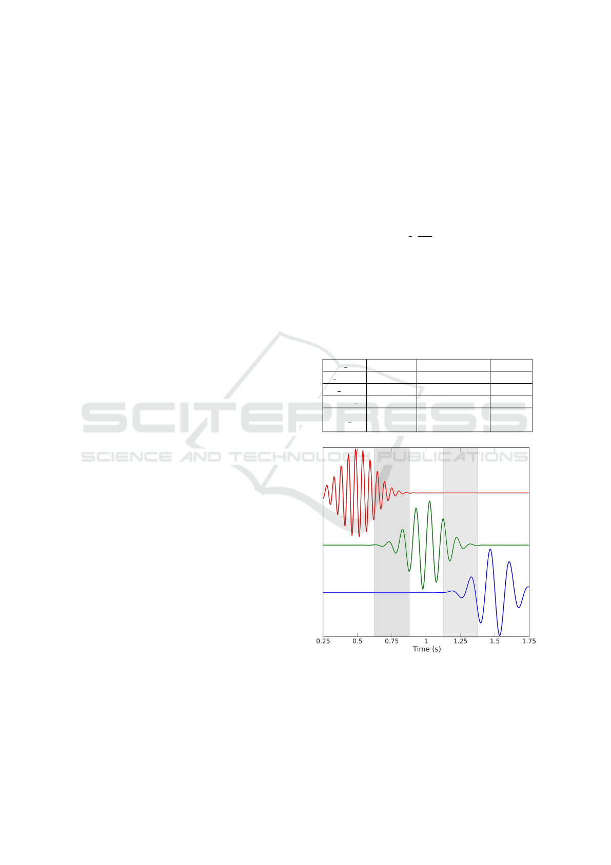
source are presented in table 1.

Table 1: Parameters for source simulation.

s i i=1 i=2 i=3

f i (Hz) 19 10 7

c i (s) 0.5 1.0 1.5

sigma i 0.12 0.12 0.12

loc i

Occipital

lobe

Sensory-motor

cortex

Frontal

lobe

Figure 1: Example of the time-courses of simulated source

activity. The light-gray shapes show the time windows

where temporal mixing is present between the sources.

Sources s

, s

, and s

are depicted in red, green, and blue

color, respectively.

Although the sources have a predeﬁned region

of the brain, the ﬁnal locations of the sources were

BIOIMAGING 2022 - 9th International Conference on Bioimaging

176

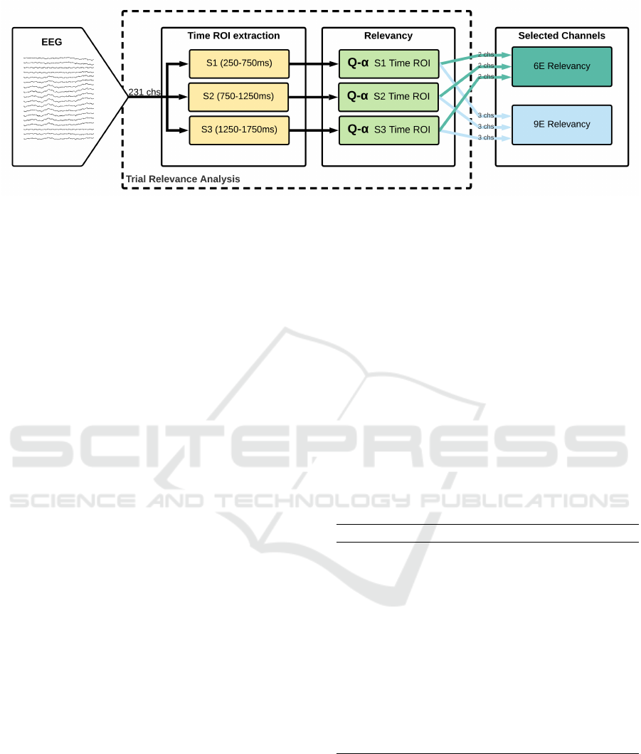
Figure 2: Relevance channel selection procedure for selecting the 6 and 9 most relevant channels per each EEG trial.

randomly selected from a set of twelve locations in

each area, distributed equally for each hemisphere.

The source ground-truth simulation process was re-

peated to obtain 150 trials with different combination

of source locations. The synthetic EEG was obtained

by using the forward equation (eq. 1), a signal-to-

noise ratio (SNR) of 0dB was added to simulate the

level of noise typically found in event related poten-

tials ERPs. An example of the ground-truth activity

can be seen in ﬁgure 1

2.4 Relevance based Channel Selection

We applied the relevance analysis proposed by (Wolf

and Shashua, 2005), to select k most relevant EEG

channels to be used for source reconstruction. A time-

ROI is selected for each source, and then for each

time-ROI, the relevance for each channel is calcu-

lated using the Standard Power-Embedded Q-α algo-

rithm. As three sources were simulated, the k =2 and

k =3 most relevant channels per each source time-ROI

were selected, therefore, the total of electrodes per

EEG used during source reconstruction for k =2 and

k =3 were 6 (we refer as Rel −6E) and 9 (we refer as

Rel −9E) respectively. In ﬁgure 2 is summarized the

selection process and presented the Time-ROI times

for each source.

By using the Standard Power-Embedded Q-α al-

gorithm, it is calculated a relevance indicator associ-

ated with each channel, this indicator is represented

by α

α ∈R(0, 1), where the values closer to 1 represent

the most relevant channels. (Wolf and Shashua, 2005)

presented the algorithm for feature selection, being

relevance directly related to the clustering quality of

features. Here, applied to EEG channel selection, the

relevance measures the ability of the channels to cap-

ture the underlying neural activity in the time-ROI.

Here the algorithm is presented in the context of EEG

channel selection. Consider the pre-processed EEG

as y

, ..., y

, such that each row is centered around

zero and its L2 norm ∣∣y

∣∣=1. For notation, the term

stands for the transpose of matrix P. Consider A

to be the afﬁnity matrix of the inner-product between

data points weighted by α

α as A

∑

i=1

. Also

consider Q

Q as an orthonormal t by k matrix, whose

columns are the k eigenvectors of A

A associated with

the highest eigenvalues. To ﬁnd the channel relevance

α is calculated by solving the optimization problem

presented below:

maxtrace

Q,α

subject to α

α =1

(3)

which can be solved by applying the Power-

Embedded Q-α algorithm (algorithm 1) adapted for

EEG channel relevance. The number of r iterations

was set to r =10 according to the number of iterations

suggested in (Wolf and Shashua, 2005).

Algorithm 1: Power-Embedded Q-α algorithm.

1: procedure Q-α(y)

2: Q

← random orthonormal q by k matrix

3: r ← 1

4: while r ≤ 10 do

5: G

i, j

← (y

r−1

6: α

α ← the largest eigenvector of G

7: A

←

∑

i=1

8: Z ← A

r−1

9: Q

R ← QR decomposition of Z

10: r ← r + 1

11: end while

12: return α

13: end procedure

2.5 Standard-based and

Coverage-based Channel

Distributions

The New York Head forward model in (Huang et al.,

2016) considers 231 electrodes positions, of which

161 are located in the scalp according to the 10-5

Relevance-based Channel Selection for EEG Source Reconstruction: An Approach to Identify Low-density Channel Subsets

177

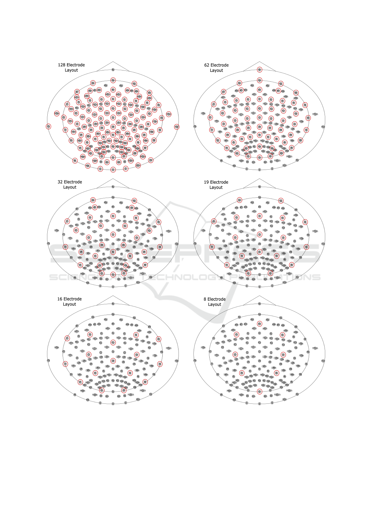
Figure 3: Standard-based (top row) and coverage-based (middle and bottom rows) electrode Layouts. The selected electrodes

for each layout are marked with a red circle over the 161 electrodes available in the New York Head.

system, and 70 electrodes distributed between neck

and face. To compare the performance of source re-

construction using relevance-based channel selection,

we selected multiple layouts based on coverage and

standard systems. One of the selected electrode dis-

tribution is based on the 161 scalp electrodes of the

BIOIMAGING 2022 - 9th International Conference on Bioimaging

178

model, we refer to it as HD−161E. Two subsets of 19

and 62 electrodes were considered based on the 10-20

and 10-10 standard electrode distribution, we refer to

them as LD −19E(10 −20) and HD −62E(10 −10),

respectively. Four more subsets of electrodes were

selected based on coverage criteria, one lays in the

category of high-density with 128 channels, it is re-

ferred as HD −128E; the other three are considered

low-density, with channel numbers of 32, 16, and 8,

they were selected trying to keep an equal coverage of

the head, they are referred as LD−32E, LD−16E, and

LD −8E. The Figure 3. shows the different standard-

based and coverage-based layouts.

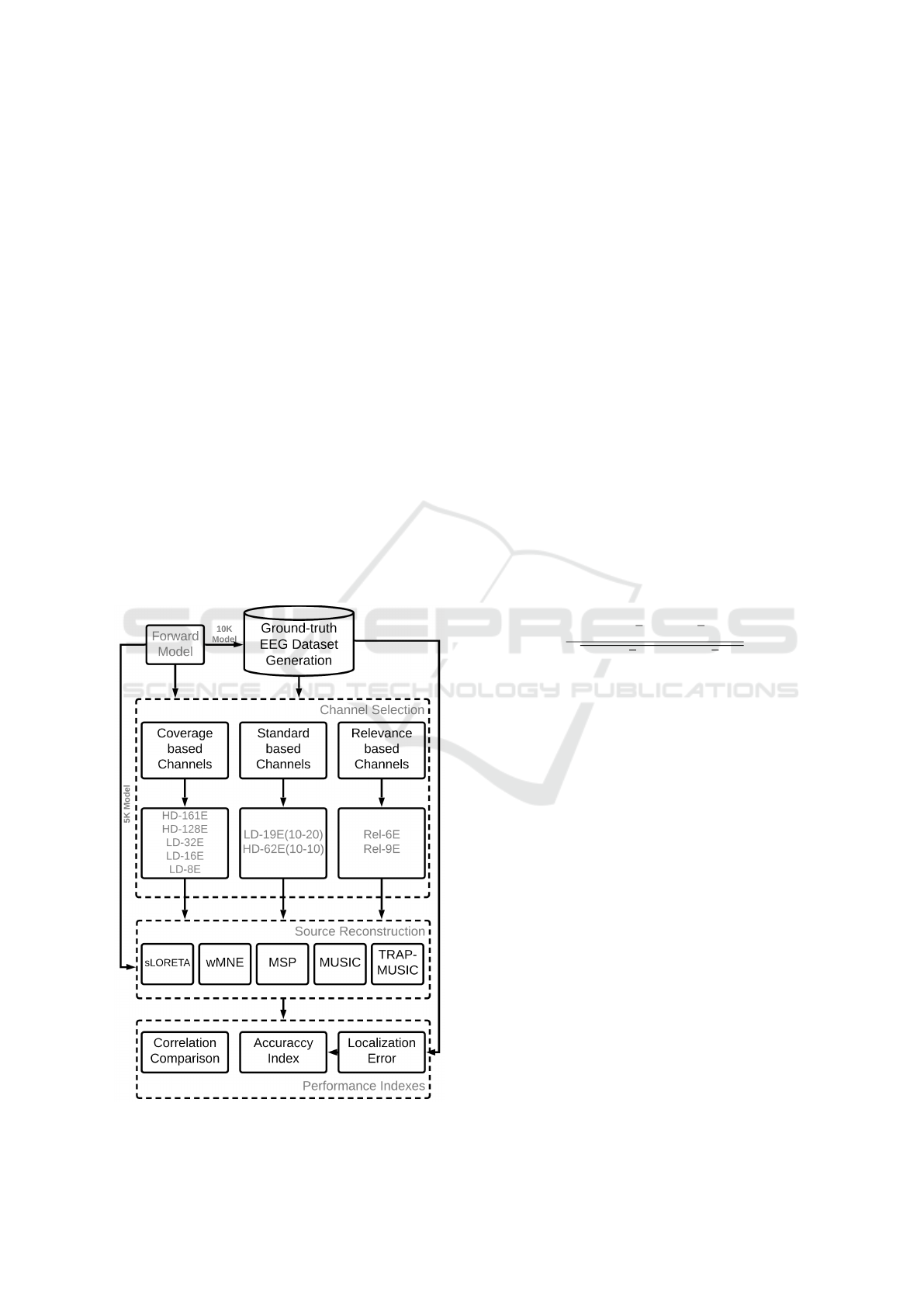
2.6 Evaluation Procedure

The evaluation procedure is presented in ﬁgure 4.

It starts with the generation of the ground-truth

EEG dataset (section 2.3). The 150 trials are pro-

cessed separately, for each EEG, the channels are

selected according to the three criteria: coverage-

based, standard-based, and relevance-based. The se-

lected channels are considered during inverse solu-

tion and processed with the ﬁve source reconstruc-

tion algorithms. The algorithms wMNE, sLORETA,

Figure 4: Summary of the evaluation procedure.

and MSP provide localization and time-course of the

sources, while MUSIC and TRAP-MUSIC provided

only source localization, however, they can be com-

plemented with Tikhonov regularization constrained

to the estimated locations to estimate the time-course

activity.

After estimating the brain activity, the localization

error for each of the three sources is calculated by us-

ing the euclidean distance (equation 4) between the

ground-truth P

and the estimated P

ˆx

location. Then,

the localization error is averaged between the three

sources to provide a single value for the error of lo-

calization.

LocE =∣∣P

−P

ˆx

∣∣

(4)

The number of trials in which the localization er-

ror with relevance selection was equal or lower than

with coverage or with standard-based layouts is pro-

posed to measure at what extend of trials, the rel-

evance selection produced equal or better accuracy

compared to the other criteria. We refer to it as the

Accuracy Comparison index.

The time course of the sources reconstructed with

Rel −6E, Rel −9E are extracted and compared with

the time courses reconstructed with the denser elec-

trode layout HD −161E. To compare them, we used

the Pearson Correlation Coefﬁcient:

r =

∑

−x

)(x

2 j

−x

2 j

)

√

∑

−x

)

∑

2 j

−x

2 j

)

(5)

where i and j are the location of the sources with the

highest amplitudes of two different reconstructions,

and x

2 j

are the time courses.

3 RESULTS

The mean and standard deviation of the localization

error for the 150 trials is shown in ﬁgure 5. The elec-

trode layouts in the x-axis were organized according

to the number of electrodes they consider, excepting

the Rel −6E and Rel −9E that were located ﬁrst on the

left side. The best accuracy was obtained when using

the highest number of electrodes with the HD−161E

layout when considering all the scalp electrodes of

the forward model. In contrast, the worst accuracy

was obtained when using the LD−8E layout. A trend

can be seen in the localization error, as the number of

electrodes is being reduced, the localization accuracy

decreases. However, the trend is abruptly interrupted

when considering the results of the channels selected

with the relevance criteria.

The localization error of the relevance selec-

tion Rel −6E and Rel −9E are comparable to the

HD −128E test. Particularly the methods wMNE,

Relevance-based Channel Selection for EEG Source Reconstruction: An Approach to Identify Low-density Channel Subsets

179

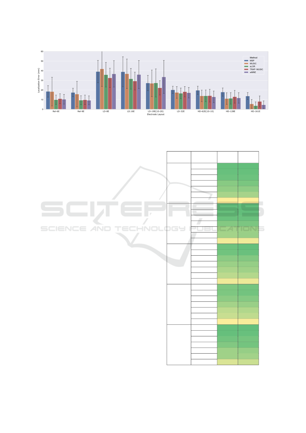
Figure 5: Localization error of the multiple electrode layouts combined with each of the source reconstruction algorithms.

sLORETA, and TRAP-MUSIC, for the relevance

cases offer a slightly better localization error mean

with similar standard deviation as with the HD −

128E. Here it is remarkable that for the same meth-

ods, Rel −9E kept the mean localization error below

10mm, result that was achieved only with all the elec-

trodes HD −161 case. The case of the MSP method

presents a similar behavior with Rel −9E compared to

HD−128E, and the MSP accuracy with Rel −9E was

slightly lower than with HD −128E. In contrast, the

MUSIC method was highly affected by the reduction

in the number of electrodes. It is a generalized effect

for this particular algorithm, regardless of whether the

channels were selected with relevance or not; as the

number of electrodes is reduced the standard devia-

tion increases.

Table 2. offers the accuracy comparison indexes

when considering the percentage of trials that ob-

tained equal or better localization error with rele-

vance criteria Rel −6E and Rel −9E, than the other

layouts based on standard and coverage criteria. It

is remarkable that for methods sLOR, wMNE, and

TRAP-MUSIC, Rel −9E obtained an index between

61% and 68% when comparing with HD −128E and

between 67% and 73% when comparing with HD −

62E(10 −10), especially considering that Rel −9E

has 119 and 51 fewer channels than HD −128E, and

HD−62E respectively. In the case of Rel −6E the re-

sults are also noticeable, it uses 122 fewer channels

than HD−128E and 55 less than HD −62E(10−10),

and it obtained indexes between 59% and 64% when

comparing with HD −128E and between 63% and

71% when comparing with HD −62E(10−10).

To compare the reconstructed time courses of the

estimated source activity, we computed the Pearson

correlation coefﬁcient between the reconstructions

using Rel −6E and Rel −9E and the denser electrode

layouts of HD −161E and HD −128E. The compari-

son was done for the reconstructions with the methods

that obtained the lowest localization error, sLORETA,

and wMNE. The results of the comparison between

Table 2: Accuracy Comparison Index, percentage of trials

that obtained equal or better localization error when com-

paring the relevance criteria Rel − 6E and Rel − 9E with

other electrode conﬁgurations.

Methods

Channel

Layout

Rel-6E Rel-9E

LD-8E 0,96 0,97

LD-16E 0,95 0,95

LD-19E 0,91 0,92

LD-32E 0,77 0,85

HD-62E 0,71 0,73

HD-128E 0,59 0,61

sLOR

HD-161E 0,11 0,11

LD-8E 0,97 0,97

LD-16E 0,95 0,97

LD-19E 0,93 0,94

LD-32E 0,79 0,84

HD-62E 0,63 0,67

HD-128E 0,62 0,68

WMN

HD-161E 0,19 0,21

LD-8E 0,91 0,97

LD-16E 0,90 0,94

LD-19E 0,75 0,80

LD-32E 0,67 0,70

HD-62E 0,57 0,64

HD-128E 0,49 0,53

MSP

HD-161E 0,21 0,22

LD-8E 0,82 0,88

LD-16E 0,83 0,89

LD-19E 0,75 0,79

LD-32E 0,62 0,68

HD-62E 0,47 0,55

HD-128E 0,42 0,47

MUSIC

HD-161E 0,13 0,15

LD-8E 0,96 0,97

LD-16E 0,96 0,95

LD-19E 0,89 0,87

LD-32E 0,81 0,88

HD-62E 0,65 0,69

HD-128E 0,64 0,63

TRAP-

MUSIC

HD-161E 0,32 0,41

BIOIMAGING 2022 - 9th International Conference on Bioimaging

180

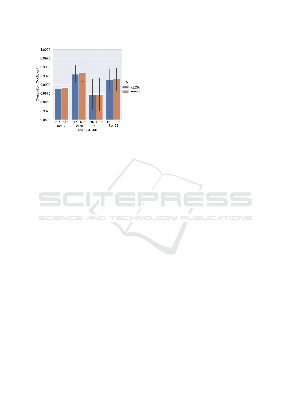
Figure 6: Source time courses correlation coefﬁcient be-

tween high-density layouts and relevance based channel se-

lection.

the aforementioned sets of channels are presented in

ﬁgure 6. It can be seen that the correlation in all

the cases was more than 98% and particularly for

the comparisons with Rel −9E, the correlation values

were higher than 99%.

To offer an overview of the relevance-based se-

lected channels we computed the number of times that

the channels were repeatedly chosen by the two rel-

evance criteria. The number of repetitions for each

channel is shown in ﬁgure 7. For relevance analysis,

the 231 channels positions of the forward model were

considered, including 70 locations in face and neck,

however, none of the selected channels were in those

areas. It is important to note that the selected chan-

nels across trials were distributed between both hemi-

spheres, in which a particular position in the right

hemisphere and its equivalent at the left hemisphere

obtained similar repetition values. The small differ-

ences can be explained by the location of the simu-

lated sources which were selected randomly from a

pre-set of sources for each brain area, equally dis-

tributed between both hemispheres.

4 DISCUSSION AND

CONCLUSIONS

With the introduction of relevance criteria for channel

selection, a subset of selected channels, with a sparser

number far from high-density EEG, can reconstruct a

set of sources in the brain with comparable quality as

a high-density number of channels. The reconstruc-

tion quality obtained with relevance channel selection

can be comparable to using a set of 128 channels, and

better than 62 channels in terms of the localization

error. Moreover, in terms of the time-courses simi-

larity, the high level of correlation obtained between

the reconstruction with the relevant channels and the

densest coverage-based layouts supports the hypothe-

sis that relevance-based channel selection criteria can

be comparable with high-density to reconstruct a par-

ticular brain activity.

The aim of this work is not to discourage the use

of high-density EEG systems, it is rather to offer an

alternative technique to select and reduce the number

of electrodes for source reconstruction while keeping

the quality. In situations where for practical reasons

high-density systems are not applicable or affordable,

low-density EEG solutions designed with relevance

criteria will favour portability and reduce the volume

of data while achieving the same quality as the high

density solutions. These traits will enable the devel-

opment of much needed EEG tools for medical di-

agnosis and non-medical applications. The results of

this research suggest the application of this analysis

in cases in which apriori known areas of the brain are

going to be monitored and it is not possible or difﬁ-

cult to constantly measure with a high-density system.

For example, in Brain-computer interfaces (BCI) sys-

tems based on source reconstructed activity (Edelman

et al., 2016; Lindgren, 2017) or Mobile Brain Imag-

ing (MoBI) applications in which the recordings are

taken out of the lab (Gramann et al., 2011; Lau-Zhu

et al., 2019).

It is important to consider that the selected elec-

trodes based on relevance criteria are relevant on the

basis of the particular source activity in which the

analysis is applied. It must not be miss-interpreted

that a selected set of electrodes can be used for map-

ping all the cortical regions. In such cases, to estimate

a generalized activity over the brain, high-density is

proven to be effective regardless of the area of the

brain activity.

It is important to note that multiple channels that

were repeatedly selected were located in positions

out of standards 10-10, and 10-20, which supports

the idea that multiple locations in non-standard posi-

tions contribute to improving the reconstruction qual-

ity, unfortunately, these positions are generally avail-

able only in denser layouts and EEG caps. However,

the use of head models including intermediate posi-

tions can be combined with the physical adjustment

of the positions of the electrodes of a system to the

relevant selected ones, in order to monitor a particu-

lar brain activity.

The proposed relevance-based channel selection

for source reconstruction remains to be veriﬁed over

real signals, further studies on multiple recording

paradigms and analysis of different brain activity re-

Relevance-based Channel Selection for EEG Source Reconstruction: An Approach to Identify Low-density Channel Subsets

181

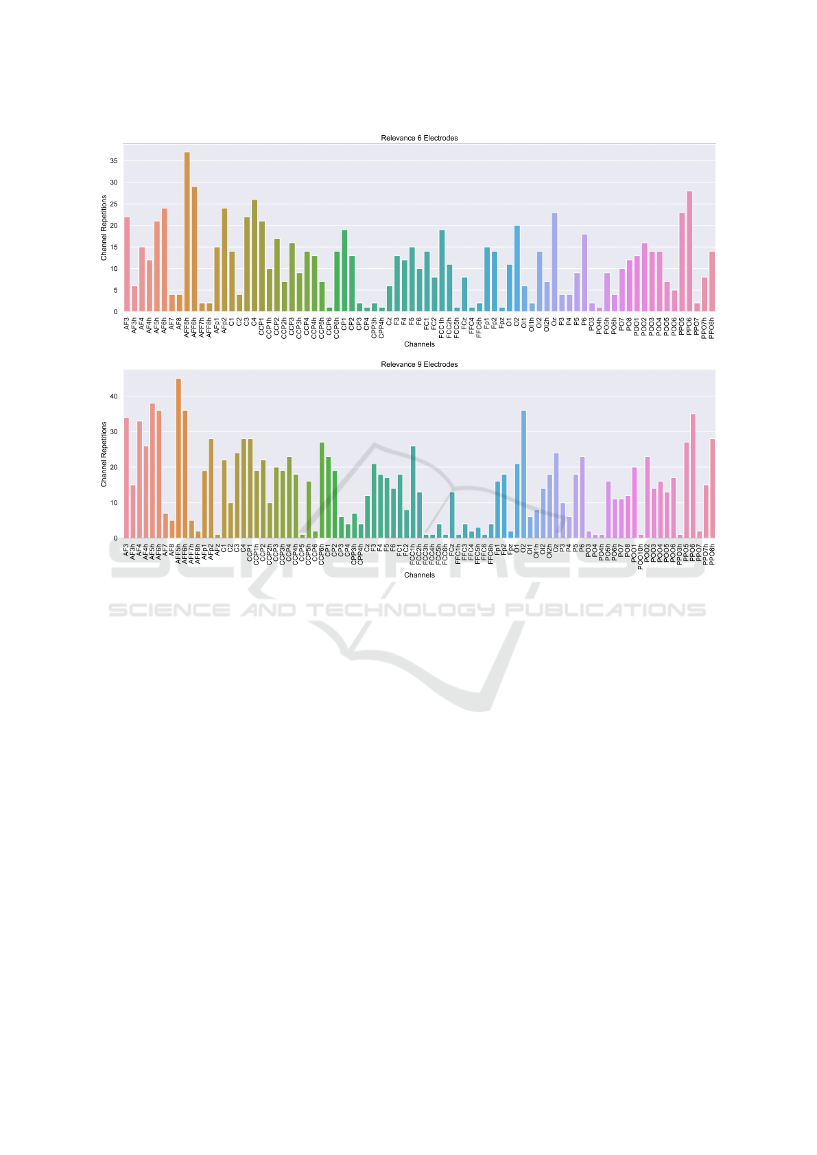
Figure 7: Channel repetition for relevance-based selection.

sponses should be done in order to validate the pro-

posed selection over a more realistic scenario. How-

ever, the presented framework for source and EEG

simulation in this study simulates signals with simi-

larities to ERPs as can be seen in ﬁgure 1. In addition,

considering that the level of noise added to the signals

had equal power than the signal, the trial data simu-

lated here can be regarded as having a similar SNR to

typical ERP signals.

In this study, we introduced the concept of rele-

vance for channel selection applied in speciﬁc time

windows (time-ROI) in which the underlying activity

was registered by the EEG recordings and compared

the performance of multiple high-density electrode

arrays, standard montages, and low-density versions

based on coverage criterion. We can conclude that the

localization accuracy and waveform of reconstructed

sources with subsets of Rel −6E and Rel −9E rel-

evant channels are comparable with reconstructions

done with coverage-based distributed sets of HD −

128 channels, and better than 62E(10 −10) channel

layout for a particular brain activity.

AUTHOR CONTRIBUTIONS

AS and EG conceived and designed the experiments.

AS performed the experiments. AF, LL, MM dis-

cussed and selected the source reconstruction algo-

rithms. All the authors analyzed the data, discussed

teh results and wrote and reﬁned the mansucript.

ACKNOWLEDGMENT

This work was supported by the Enabling technology

program of Biotechnology of Norwegian University

of Science and Technology NTNU, project ”David

and Goliath: single-channel EEG unravels its power

through adaptive signal analysis”.

REFERENCES

(1961). The ten twenty electrode system: International fed-

eration of societies for electroencephalography and

BIOIMAGING 2022 - 9th International Conference on Bioimaging

182

clinical neurophysiology. American Journal of EEG

Technology, 1(1):13–19.

Chatrian, G. E., Lettich, E., and Nelson, P. L. (1985).

Ten percent electrode system for topographic studies

of spontaneous and evoked eeg activities. American

Journal of EEG Technology, 25(2):83–92.

Colton, D. and Kress, R. (2019). Inverse Acoustic and Elec-

tromagnetic Scattering Theory. Springer, 4 edition.

Edelman, B. J., Baxter, B., and He, B. (2016). Eeg source

imaging enhances the decoding of complex right-hand

motor imagery tasks. IEEE Transactions on Biomedi-

cal Engineering, 63:4–14.

Friston, K., Harrison, L., Daunizeau, J., Kiebel, S., Phillips,

C., Trujillo-Barreto, N., Henson, R., Flandin, G., and

Mattout, J. (2008). Multiple sparse priors for the

M/EEG inverse problem. NeuroImage, 39(3):1104–

1120.

Gramann, K., Gwin, J. T., Ferris, D. P., Oie, K., Jung, T.-P.,

Lin, C.-T., Liao, L.-D., and Makeig, S. (2011). Cogni-

tion in action: imaging brain/body dynamics in mobile

humans. 22(6):593–608.

Hallez, H., Vanrumste, B., Grech, R., Muscat, J., De Clercq,

W., Vergult, A., D’Asseler, Y., Camilleri, K. P., Fabri,

S. G., Van Huffel, S., and Lemahieu, I. (2007). Re-

view on solving the forward problem in EEG source

analysis. Journal of NeuroEngineering and Rehabili-

tation, 4.

ainen, M. S. and Ilmoniemi, R. J. (1994). Interpret-

ing magnetic ﬁelds of the brain: minimum norm esti-

mates. Medical & Biological Engineering & Comput-

ing, 32(1):35–42.

Huang, Y., Parra, L. C., and Haufe, S. (2016). The new

york head—a precise standardized volume conduc-

tor model for eeg source localization and tes target-

ing. NeuroImage, 140:150 – 162. Transcranial electric

stimulation (tES) and Neuroimaging.

Ilmoniemi, R. J. and Sarvas, J. (2019). Brain Signals:

Physics and Mathematics of MEG and EEG. The MIT

Press.

Iwaki, S. and Ueno, S. (1998). Weighted minimum-norm

source estimation of magnetoencephalography utiliz-

ing the temporal information of the measured data.

Journal of Applied Physics, 83(11):6441.

Jasper, H. (1958). Ten-Twenty Electrode System of the In-

ternational Federation. Electroencephalography and

Clinical Neurophysiology, 10:371–375.

Jatoi, M. A. and Kamel, N. (2018). Brain source localiza-

tion using reduced eeg sensors. Signal, Image and

Video Processing, 12(8):1447–1454.

Jatoi, M. A., Kamel, N., Malik, A. S., Faye, I., and Be-

gum, T. (2014). A survey of methods used for source

localization using eeg signals. Biomedical Signal Pro-

cessing and Control, 11:42 – 52.

Lau-Zhu, A., Lau, M. P., and McLoughlin, G. (2019). Mo-

bile EEG in research on neurodevelopmental disor-

ders: Opportunities and challenges. Developmental

Cognitive Neuroscience, 36:100635.

Lindgren, J. T. (2017). As above, so below? Towards un-

derstanding inverse models in BCI. Journal of Neural

Engineering, 15(1):012001.

akel

a, N., Stenroos, M., Sarvas, J., and Ilmoniemi, R. J.

(2018). Truncated RAP-MUSIC (TRAP-MUSIC) for

MEG and EEG source localization. NeuroImage,

167:73–83.

Michel, C. M. and Brunet, D. (2019). EEG source imaging:

A practical review of the analysis steps. Frontiers in

Neurology, 10(APR):325.

Mosher, J. C. and Leahy, R. M. (1998). Recursive MU-

SIC: A framework for EEG and MEG source localiza-

tion. IEEE Transactions on Biomedical Engineering,

45(11):1342–1354.

O’Leary, J. (1970). Hans berger on the electroencephalo-

gram of man. the fourteen original reports on the hu-

man electroencephalogram. translated from the ger-

man and edited by pierre gloor. Science, 168:562–563.

Oostenveld, R. and Praamstra, P. (2001). The ﬁve

percent electrode system for high-resolution EEG

and ERP measurements. Clinical Neurophysiology,

112(4):713–719.

Pascual-Marqui, R. D. (2002). Standardized low-resolution

brain electromagnetic tomography (sLORETA): Tech-

nical details. Methods and Findings in Experimental

and Clinical Pharmacology, 24(SUPPL. D):5–12.

Phillips, J. W., Leahy, R. M., Mosher, J. C., and Timsari,

B. (1997). Imaging neural activity using MEG and

EEG. IEEE Engineering in Medicine and Biology

Magazine, 16(3):34–42.

Seeck, M., Koessler, L., Bast, T., Leijten, F., Michel, C.,

Baumgartner, C., He, B., and Beniczky, S. (2017). The

standardized EEG electrode array of the IFCN.

Sohrabpour, A., Lu, Y., Kankirawatana, P., Blount, J., Kim,

H., and He, B. (2015). Effect of EEG electrode num-

ber on epileptic source localization in pediatric pa-

tients. Clinical Neurophysiology, 126(3):472–480.

Soler, A., Giraldo, E., and Molinas, M. (2020a). Low-

density EEG for Source Activity Reconstruction us-

ing Partial Brain Models. In Proceedings of the

13th International Joint Conference on Biomedical

Engineering Systems and Technologies, pages 54–63.

SCITEPRESS - Science and Technology Publications.

Soler, A., Mu

noz-Guti

errez, P. A., Bueno-L

opez, M., Gi-

raldo, E., and Molinas, M. (2020b). Low-Density

EEG for Neural Activity Reconstruction Using Mul-

tivariate Empirical Mode Decomposition. Frontiers in

Neuroscience, 14:175.

Song, J., Davey, C., Poulsen, C., Luu, P., Turovets, S., An-

derson, E., Li, K., and Tucker, D. (2015). EEG source

localization: Sensor density and head surface cover-

age. Journal of Neuroscience Methods, 256:9–21.

Wolf, L. and Shashua, A. (2005). Feature Selection for

Unsupervised and Supervised Inference: The Emer-

gence of Sparsity in a Weight-Based Approach * Am-

non Shashua. Journal of Machine Learning Research,

6:1855–1887.

Relevance-based Channel Selection for EEG Source Reconstruction: An Approach to Identify Low-density Channel Subsets

183