
Improving the Efficiency of Autoencoders for Visual Defect Detection
with Orientation Normalization
Rich
´
ard R
´
adli and L
´
aszl
´
o Cz
´
uni
a
Faculty of Information Technology, University of Pannonia, Egyetem Street 10., Veszpr
´
em, Hungary
Keywords:
Autoencoder Neural Network, Convolutional Neural Network, Defect Detection, Unsupervised Anomaly
Detection, Spatial Transformer Network.
Abstract:
Autoencoders (AE) can have an important role in visual inspection since they are capable of unsupervised
learning of normal visual appearance and detection of visual defects as anomalies. Reducing the variability of
incoming structures can result in more efficient representation in latent space and better reconstruction quality
for defect free inputs. In our paper we investigate the utilization of spatial transformer networks (STN) to
improve the efficiency of AEs in reconstruction and defect detection. We found that the simultaneous training
of the convolutional layers of the AEs and the weights of STNs doesn’t result in satisfactory reconstructions
by the decoder. Instead, the STN can be trained to normalize the orientation of the input images. We evaluate
the performance of the proposed mechanism, on three classes of input patterns, by reconstruction error and
standard anomaly detection metrics.
1 INTRODUCTION
The visual inspection of products is often inevitable
in many manufacturing processes. Since anomalous
items are often missing during the training process
unsupervised anomaly detection is the most suitable
approach to build a defect detection system. In our
paper we are to improve autoencoder (AE) neural
networks to reach better model generation at given
convolutional complexity and latent space size. As
a consequence we expect better accuracy to detect
anomalies. It is already shown that denoising AEs can
perform better than base AEs in anomaly detection
(R
´
adli and Cz
´
uni, 2021), and that applying structural
similarity in the loss function during training can also
improve results (Bergmann et al., 2018). Now, our
idea is to apply geometric transformations to normal-
ize the rotation of the input images, thus AE can more
efficiently compress and reconstruct input patterns.
In Section 2 we introduce autoencoders, in Sec-
tion 3 we discuss the usage of AEs for anomaly de-
tection, while in Section 4 the operation of spatial
transformer networks (STNs) (Jaderberg et al., 2015)
is described. The combination of AEs with STNs is
discussed in Section 5. The proposed normalization
technique can be found in Section 6 and the dataset
used in experiments are introduced in 7. Results are
a
https://orcid.org/0000-0001-7667-9513
discussed in Section 8 and finally conclusions and fu-
ture work are given in 9.
2 DIFFERENT TYPES OF
AUTOENCODERS
AEs are defined as feed-forward neural networks
containing three main sequential components:
the encoder network E : R
k×h×w
→ R
d
, the latent
space R
d
, and the decoder network D : R
d
→ R
k×h×w
.
ˆ
x = D(E(x)) = D(z),
(1)
where x is the input data, z is the latent information,
and
ˆ
x is the output of the network. Their similarity to
principal component analysis (PCA) is well known,
moreover, AEs could outperform linear or kernel
PCAs in many cases (Sakurada and Yairi, 2014) .
AEs can be categorized according to their loss
functions. The loss function (J), to learn a specific
task, can be generally formed this way:
J(x, ω) =
1
n
∑
kx −
ˆ
xk + R(z),
(2)
where ω = (w
E
, b
E
, w
D
, b
D
) are the weights and
biases of the encoder and decoder networks and n is
Rádli, R. and Czúni, L.
Improving the Efficiency of Autoencoders for Visual Defect Detection with Orientation Normalization.
DOI: 10.5220/0010903600003124
In Proceedings of the 17th International Joint Conference on Computer Vision, Imaging and Computer Graphics Theory and Applications (VISIGRAPP 2022) - Volume 4: VISAPP, pages
651-658
ISBN: 978-989-758-555-5; ISSN: 2184-4321
Copyright
c
2022 by SCITEPRESS – Science and Technology Publications, Lda. All rights reserved
651

the number of elements in a batch. In sparse AEs R
is based on the Kullback-Leibler divergence or on the
L1 norm, the purpose is to make the most of the hid-
den unit’s activations close to zero. Contractive AEs
apply the Frobenius norm on the derivative of z as
a function of x to make the model resistant to small
perturbations; in an information theoretic-learning
autoencoder Renyi’s entropy is used; while feature
matching autoencoders (Dosovitskiy and Brox, 2016)
enforce the features of the input and its reconstruction
to be equal:
J(x,
˜
x, ω) = w
im
∑
(x −
ˆ
x)
2
+ w
f t
∑
(F(x) − F(
ˆ
x))
2
,
(3)
where F is a feature extractor which can be fixed
or also trained. The SSIM-AE (Bergmann et al.,
2018) can be considered as a kind of feature matching
AEs (Eq. 3) where the loss function utilizes the struc-
tural similarity (Wang et al., 2004) of images repre-
senting, beside luminance, local variance and covari-
ance. The denoising autoencoder (DAE) is an exten-
sion of the basic autoencoder, which is trained to re-
construct corrupted input data. C denotes the corrupt-
ing function generating
˜
x. Eq. 1 now becomes:
ˆ
x = D(E(C(x))) = D(E(
˜
x)) = D(z).
(4)
The applied loss can weight between untouched and
artificially corrupted areas. Variational AEs (VAEs)
impose constraints on the latent variables in a differ-
ent way, they estimate posteriori probability p(z|x)
with an assumption of a prior knowledge p(z) be-
ing a normal Gaussian distribution. Adversarial AEs
(AAEs) use generative adversarial networks (GANs)
to perform variational inference. VAEs and AAEs are
both generative models, and both are based on max-
imum likelihood. The difference between VAEs and
AAEs can be characterized that while VAEs apply ex-
plicit rules on z, AAEs control its distribution implic-
itly.
3 ANOMALY DETECTION WITH
AUTOENCODERS
AEs are among the candidates for unsupervised
anomaly detection in industrial applications, their re-
cent performance ranks them in the middle of the
state-of-the-art (Bergmann et al., 2021). Our purpose
is to find ways to improve the detection accuracy of
baseline AEs. The detection of faults in images is
typically solved by computing the difference between
the input and the decoded signal. If it is above a given
threshold T , we set the detection map to 1:
m =
(
1, if ||x −
ˆ
x|| > T,
0, otherwise.
(5)
The applied ||.|| can be various (e.g. L
1
, L
2
, SSIM
(Bergmann et al., 2018)).
In (Beggel et al., 2019) authors deal with the prob-
lem of training AEs when the training set is contami-
nated with some outliers. Their proposed adversarial
autoencoder imposes a prior distribution on the latent
representation, placing anomalies into low likelihood
regions, thus potential anomalies can be identified and
rejected already during training. (Tuluptceva et al.,
2020) proposes perceptual deep autoencoders where
relative-perceptual-L1 loss (Tuluptceva et al., 2020),
robust to low contrast and noise, is applied for train-
ing and also to predict the abnormality for new inputs.
In (Alaverdyan et al., 2020) an unsupervised siamese
autoencoder is proposed to detect anomalies in brain
MRI images by a one class SVM in latent space. The
role of the siamese network is to regularize the latent
space: R(z) (Eq. 2) is the cosine distance of two in-
dependent samples in the two siamese branches in the
latent space. In (R
´
adli and Cz
´
uni, 2021) blocks of
pixels were deleted as simulated noise in a denoising
SSIM-AE, and the SSIM-AE was forced to learn the
reconstruction of areas from neighboring territories;
this strategy resulted in better anomaly detection for
different classes of inputs when compared to the base
SSIM-AE.
The improvement of VAEs with STNs was pub-
lished in (Bidart and Wong, 2019) but there were
questions raised regarding the simultaneous learning
of VAE and STN weights, and its effect on anomaly
detection was not investigated at all. These are our
main questions in this article but we use AEs (instead
of VAEs) as the base, starting model.
For a deeper review on AEs and their application
we propose to check paper (Zhai et al., 2018).
3.1 The AE Framework in Our Study
Table 1 contains our autoencoder following the struc-
ture of (Bergmann et al., 2018) but applying squared
difference (L
2
) in the loss function instead of SSIM.
While the complexity of this structure could be im-
proved with success (such can be found in (R
´
adli and
Cz
´
uni, 2021)) but this convolutional AE can serve
as a good base model for our comparisons. The de-
coder part is simply building up the input image in a
symmetrical structure to the encoder using deconvo-
lutions.
VISAPP 2022 - 17th International Conference on Computer Vision Theory and Applications
652

Table 1: Architecture of the applied encoder for input image
128 × 128 × 3. d = 100 for the texture and screw images.
Layer Output Size Kernel Stride Padding
Input 128x128x3
Conv1 64x64x32 4x4 2 1
Conv2 32x32x32 4x4 2 1
Conv3 32x32x32 3x3 1 1
Conv4 16x16x64 4x4 2 1
Conv5 16x16x64 3x3 1 1
Conv6 8x8x128 4x4 2 1
Conv7 8x8x64 3x3 1 1
Conv8 8x8x32 3x3 1 1
Conv9 1x1xd 8x8 1 0
4 SPATIAL TRANSFORMER
NETWORKS
Spatial transformer networks (STN) were proposed
by (Jaderberg et al., 2015), designed for the spatial
transformation of data within existing network archi-
tectures. It was shown that the use of the spatial trans-
formers results in models which learn invariance to
translation, scale, rotation and more generic warp-
ings, leading to state-of-the-art performance on sev-
eral benchmarks. STN consists of three main parts:
• Localisation subnetwork: its task is to figure out
the right transformation parameters θ. It can have
any form but should include a final regression
layer to produce the transformation parameters.
(Typically affine and perspective transformations
are in focus but in our study we focus only on ro-
tations as discussed later.)
• Sampling grid generator: to perform the geomet-
ric transformation of the input, each output value
should be computed by applying a sampling ker-
nel centered at a particular location in the input.
The sampling grid defines how to compute the lo-
cations of values on the input.
• Sampler: this part computes the result of transfor-
mation sampling the input according to the sam-
pling grid.
Figure 1: The base STN architecture, where U is the input
image or image features, and V is the transformed version
of them.
STNs are found to be useful in the improvement
of many classical image processing tasks. For ex-
ample in (Li et al., 2018) the recognition of jersey
numbers in soccer videos was improved by adding
STN to the front end of a classification network. To
help the learning phase, a semi-supervised mecha-
nism was proposed, where the localisation error was
part of the loss function, beside softmax classifica-
tion loss. In (Lee et al., 2019) the goal was to learn
a complex function that maps the appearance of input
image pairs to the parameters of the spatial transfor-
mation in order to register anatomical structures. To
guide the registration of the moving image to the fixed
one, alternatives of the loss function contained pre-
pared structures-of-interest regions (segmentations or
landmarks) beside the pixel-wise registration error.
Discussing all applications are beyond our paper,
there are interesting ones, such as grasp detection
(Park and Chun, 2018), image retrieval (Ding et al.,
2020), or change detection (Chianucci and Savakis,
2016). The most similar paper to ours is (Bidart and
Wong, 2019), where VAE networks were extended
with STNs. Their findings are discussed in the next
section.
5 STNs WITH AUTOENCODERS
It seems straightforward that the insertion of an STN
at the front end of an AE and the inverse transfor-
mation after the decoder can result in better recon-
struction, since the STN might learn the best spatial
transformation warping images to similar scale, po-
sition, and orientation. This way the AE meets less
variability of input patterns, can more easily learn the
necessary convolutions, and finally can make a better
reconstruction. Figure 2 illustrates this configuration.
Figure 2: STN inserted into an AE with the inverse spatial
transformation.
Unfortunately, to simultaneously find the optimal
weights for either the localisation network and the AE
is not guaranteed. In (Bidart and Wong, 2019) the
same structure was used but instead of AE a VAE was
used. We quote the description of this problem from
(Bidart and Wong, 2019): ”We find in practice there
are issues with the optimizer being caught in local
minima, so we use multiple random restarts, where
Improving the Efficiency of Autoencoders for Visual Defect Detection with Orientation Normalization
653
we first try the loss at a set number of affine param-
eters, and only perform gradient descent on the best
performing parameters.” Moreover, they investigated
only images from the MNIST database of handwrit-
ten digits, which are almost binary patterns from a
small size set of classes. Also, it is a question how
the combination of STNs and AEs perform in case of
more complicated structures (such as grayscale tex-
tures for example) and what effect does all these have
on anomaly detection. Since our AEs are fully con-
volutional and test images have the same scale, only
the orientation of input patterns should be compen-
sated by the STN, we can avoid the learning of trans-
lation and scaling parameters. Fig. 3 illustrates typ-
ical learning curves for our pure AE (given in Sub-
section 3.1) and the one extended with the STN (as
illustrated by Fig. 2). Interestingly, in this example
Figure 3: Learning curves for AE and STN+AE for the class
Texture 1.
the inclusion of STN resulted in even higher loss val-
ues; the same happened with many other test images.
Thus the inclusion of STN did not improve the perfor-
mance of the AE. Looking for the reason of this per-
formance drop we found that the widely used Keras
implementation (STN, 2016) of the STN has low ac-
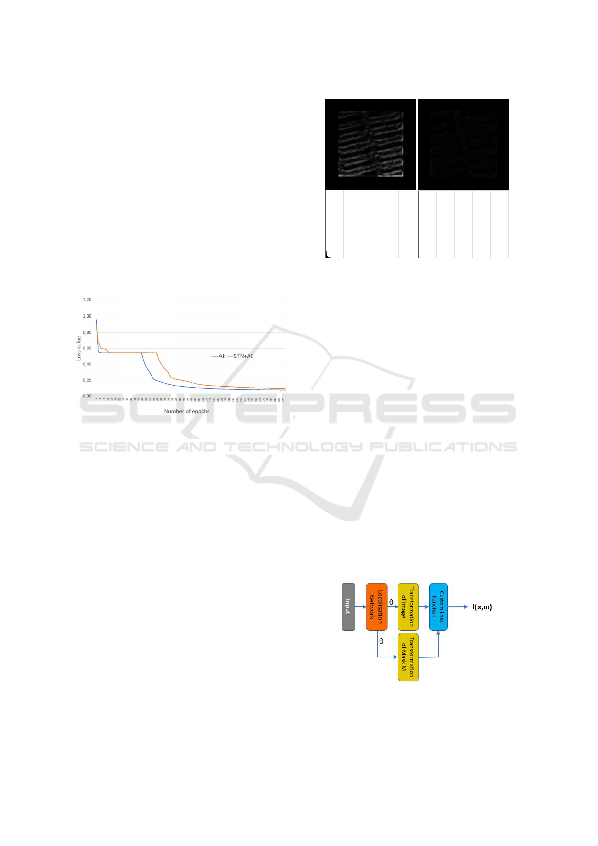
curacy. Fig. 4 illustrates the differences, when an
image was rotated by 45°and then back to its original
orientation. The error of interpolation computed with
code (STN, 2016) is very high (see Fig. 4 left). This
means that the inverse spatial transformation, after the
decoding step, will not accurately reproduce the same
orientation of the input and it will result in a larger
value in Eq. 5. To get rid of this transformation error
we replaced the grid generator and sampler of (STN,
2016) with the built in spatial transformation function
of TensorFlow (tfa.image.transform). As can be seen
on Fig. 4 right this implementation gives almost per-
fect inverse transformation.
To investigate the simultaneous optimization of AE
and STN weights we tested three strategies:
• We started both STN and AE with random
weights and the loss function used the square
Figure 4: Example for rotation and inverse rotation of a
Texture 1 image with 45°. Left: the difference image (be-
tween input and inverse rotated) shows inaccurate compu-
tations in the STN implementation (STN, 2016). Right:
the same difference image when rotations and their inverse
were performed by built in TensorFlow function, called
tfa.image.transform. In the second row the histograms are
given for better illustration.
function in Eq. 1 without any regularization
(R = 0).
• We separated the STN from the AE during train-
ing. STN was pre-trained to normalize the orien-
tation of input patterns as detailed in the following
section. During the training of the AE the locali-
sation network was frozen.
• The same as above but allowed the training to re-
fine the weights of the STN.
In the next Section we discuss the case of pre-trained
STNs.
6 NORMALIZATION WITH STNs
The purpose of normalization STN is to rotate the in-
puts to the same orientation. To achieve this we built
an STN where the loss function is based on image
gradients.
Figure 5: STN with custom loss function as specified by Eq.
7.
VISAPP 2022 - 17th International Conference on Computer Vision Theory and Applications
654
Local image gradients were computed with a con-
volution kernel on the re-scaled variant (64 × 64) of
the image. To sub-press image noise and small de-
tails, Gaussian blur was applied before computing the
horizontal gradients by the vertical Sobel filter:
G
x
=
−1 0 +1
−2 0 +2
−1 0 +1
(6)
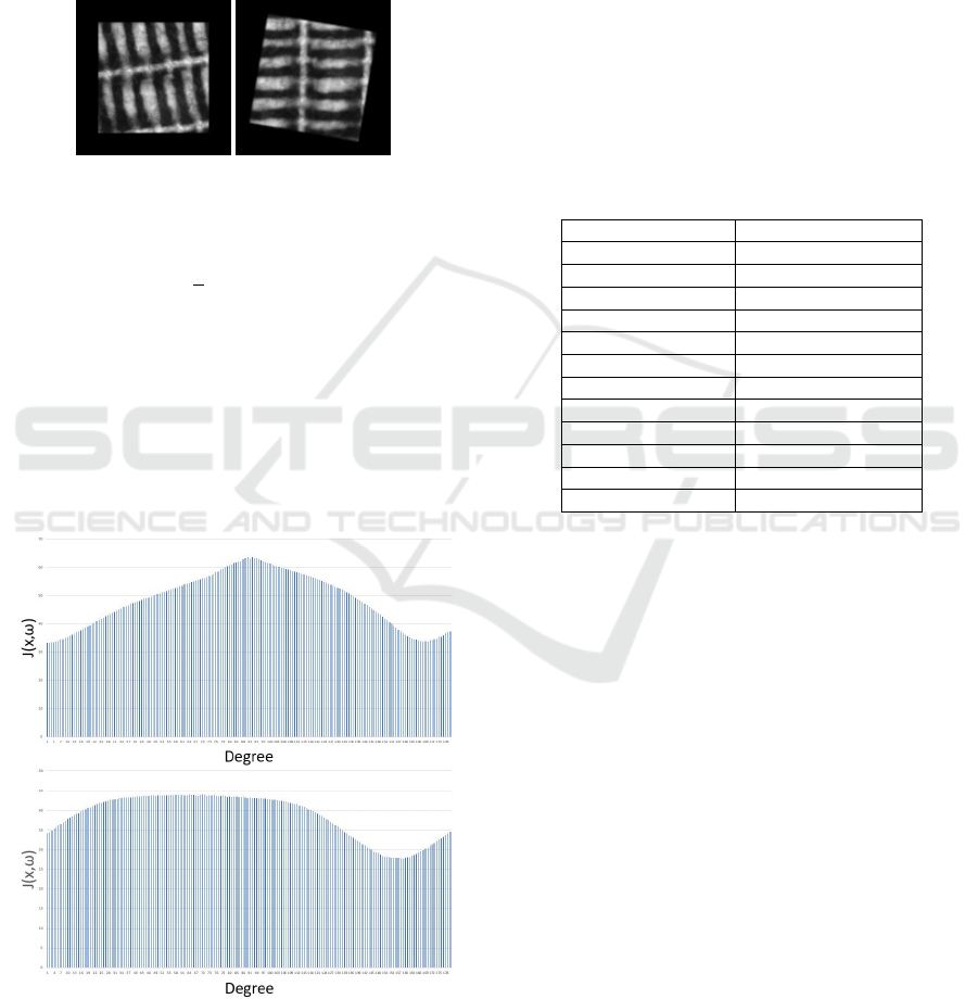
Figure 6: Input image from class Texture 1 with 0 padding
and its rotated version.
The loss function of the STN is defined as:
J(x, ω) =
1
n
∑
|(M ◦
ˆ
x) ~ G
x
|,
(7)
where
ˆ
x is the output of the STN network, and M is a
rotated mask for the central region of the 0 padded im-
age. The 0 padding is necessary to avoid losing infor-
mation when some parts of the rotated image lay out-
side the original frame. See illustration in Fig. 6. The
element-wise product with M is to get rid of possible
high gradient areas where the padding region meets
the central content.
Figure 7: Illustrations for the loss value for two images from
class Texture 1 at different rotation angles.
Fig. 7 illustrates the loss values for two images
from the Texture 1 class. In the top example we can
see that there are two minima of the function with ap-
proximately 10 degrees difference but both functions
are quite smooths. This means that we don’t expect
to find always exactly the same orientation but the
smoothness of the function and the differentiability
of STNs (Jaderberg et al., 2015) can result almost the
same orientation.
6.1 The Localisation Network
There is no specific rule about the architecture of a
localisation network (except for its final regression
layer), fundamentally, it can be either a convolutional
neural network or a fully connected network. The ar-
chitecture of our localisation network can be seen in
Table 2.
Table 2: Architecture of the localisation network.
Name of the layer Activation function
Convolution 1 Relu
MaxPool 1 None
Convolution 2 Relu
MaxPool 2 None
Convolution 3 Relu
MaxPool 3 None
Convolution 4 Relu
MaxPool 4 None
Flatten None
Fully-connected 1 Relu
Fully-connected 2 Relu
Fully-connected 3 None
Its task is to obtain the θ matrix which holds the
parameters of spatial transformation. As explained
above, in our implementation, we limited θ to rota-
tions, that is:
θ =
cos(α) −sin(α) 0
sin(α) cos(α) 0
(8)
As for the θ
−1
, we simply extend the transforma-
tion matrix with a row of [0,0,1] and calculate the in-
verse, followed by the cropping the unnecessary row.
For training the STN we feeded 10,000 images to the
network (80% for training, 20% for validation). The
image size was set to 128 × 128. The network was
trained for 50 epochs, using the ADAM optimizer,
where the learning rate was set to 2 × 10
−4
, while the
value of the weight decay was 10
−5
. At the end of the
training, we saved the weights of the network for later
utilization.
7 DATASETS
To evaluate to performance of the autoencoders we
used three datasets: the two texture image sets (Tex-
Improving the Efficiency of Autoencoders for Visual Defect Detection with Orientation Normalization
655
ture 1 and Texture 2) were provided by (Bergmann
et al., 2018), while the Screw class is from (Bergmann
et al., 2019). The original texture sets included 100-
100 defect-free images, and 50-50 defective images,
with various faults. Pixel-wise ground truth images
were also provided by the authors. All of the origi-
nal texture images are of the size of 512× 512 pixels.
The Screw class has 320 defect-free images of size
1024 × 1024; the defective class Thread-top, used in
our defect detection tests, has 23 images. First im-
ages were resized to 256 × 256 pixels, then patches
of size 128 × 128 were created. At this point, we ap-
plied various augmentation procedures such as rota-
tions and cropping. It is vital in order to enrich our
dataset. Then we added 0 padding with the minimally
necessary size to avoid clipping the content when ro-
tating them by the STN: this resulted in an image size
of 181 × 181 pixels. Finally, these images were re-
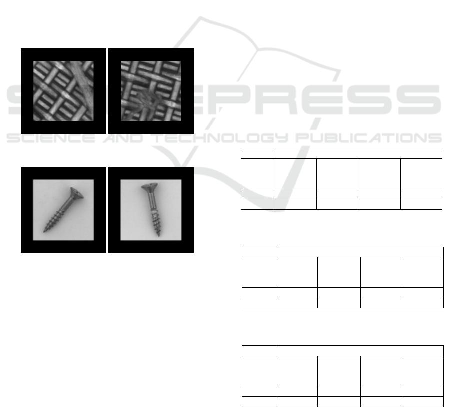
sized to 128 × 128. For the illustration of the three
classes see Fig. 6, Fig. 8, and Fig. 9, each class
contained finally 10,000 images used for training and
validation.
Figure 8: Test images from the Texture 2 dataset.These ex-
amples shows some defects to be detected.
Figure 9: Train and test images from the Screw dataset.
8 TESTS AND DISCUSSIONS
In this section we first investigate the reconstruction
abilities of the differently trained variants of the struc-
ture given in Section 5 and illustrated by Fig. 2. It has
already been shown in (R
´
adli and Cz
´
uni, 2021) that
higher reconstruction accuracy does not strictly im-
ply better detection rates that is the reason we also
run tests for their application for defect detection.
8.1 Testing the Reconstruction
Accuracy
Four cases are under investigation:
1. For reference we trained the plain AE defined in
Section 3.1.
2. Both STN and AE are initialized with random
weights.
3. STN is pre-trained to normalize the orientation of
input patterns. During the training of the AE the
localisation network is frozen.
4. The same as above but allowing the refinement of
STN weights.
These four cases correspond to the four columns
in Table 3, 4, and 5, where SSIM and mean squared
error (MSE) values are computed as the mean of 2000
test images. (Lower MSE and higher SSIM mean bet-
ter quality). Hyper parameters were exactly the same
in all cases: Networks were trained on NVIDIA RTX
5000 GPU for 200 epochs with ADAM optimizer, ini-
tial learning rate was 2 × 10
−4
with 10
−5
weight de-
cay. The latent space was set to d = 100. All exper-
iments were repeated 5 times, data given are average
values. (Abbreviations in Table 3, 4, 5, 6, 7, 8 and 9
are the following: S: STN; rnd. in. S w.: randomly
initialized STN weights; pre-tr. frz. S w.: pre-trained
frozen STN weights; pre-tr. n. frz. S w.: pre-trained
not frozen STN weights.)
Table 3: Reconstruction quality of images of the class Tex-
ture 1. Abbreviations are given in the text.
Texture 1
AE
S+AE
pre-tr.
frz. S w.
S+AE
rnd. in.
S w.
S+AE
pre-tr. n.
frz. S w.
MSE 82.4781 77.1195 83.0611 74.8105
SSIM 0.8453 0.8790 0.8411 0.8883
Table 4: Reconstruction quality of images of the class Tex-
ture 2. Abbreviations are given in the text.
Texture 2
AE
S+AE
pre-tr.
frz. S w.
S+AE
rnd. in.
S w.
S+AE
pre-tr. n.
frz. S w.
MSE 88.3534 86.1341 89.9087 87.9534
SSIM 0.7915 0.8174 0.7675 0.7911
Table 5: Reconstruction quality of images of the class
Screw. Abbreviations are given in the text.
Screw
AE
S+AE
pre-tr.
frz. S w.
S+AE
rnd. in.
S w.
S+AE
pre-tr. n.
frz. S w.
MSE 36.2071 34.2324 37.7939 35.2554
SSIM 0.8729 0.9075 0.8707 0.8893
VISAPP 2022 - 17th International Conference on Computer Vision Theory and Applications
656

In accordance with the observation of (Bidart and
Wong, 2019), quoted in Section 5, we found that in
all three image classes the insertion and random ini-
tialization of the STN (and the insertion of the corre-
sponding inverse transformation) could not improve
reconstruction quality, in all cases we got worse re-
sults. Pre-training the STN with the method intro-
duced in Section 6 resulted in improved quality com-
pared to the plain AE. Moreover, allowing the fine-
tuning of STN weights, simultaneously with the train-
ing of the AE resulted in lower quality in two cases of
the three.
8.2 Defect Detection
For the further evaluation of the proposed method
we tested defect detection using the ground truth
defect images of the sources named in Section 7.
Three well-known pixel-level metrics were used
for comparisons: receiver operating characteristic
(ROC) curves, precision-recall curves (PRC), and
intersection over union (IoU). In case of all curves
the area under curve (AuC) was calculated. Residual
maps (between the inputs and the decoded and
inverse transformed outputs) were created using both
SSIM and MSE with different thresholding, resulting
in the above mentioned curves. The differences were
computed only on the central regions of the padded
test images (excluding the 0 padding areas).
Table 6: Defect detection using SSIM and MSE metrics for
the Texture 1 class. Abbreviations are given in the text.
Texture 1
AE
S+AE
pre-tr.
frz. S w.
S+AE
rnd. in
S w.
S+AE
pre-tr. n.
frz S w.
SSIM
ROC 0,8622 0,8752 0,8591 0,8712
PRC 0,3996 0,3993 0,3882 0,4008
IoU 0,1228 0,1228 0,1228 0,1227
MSE
ROC 0,6514 0,6694 0,6635 0,6672
PRC 0,2007 0,2229 0,2093 0,2215
IoU 0,0744 0,0796 0,0768 0,0803
Table 7: Defect detection using SSIM and MSE metrics for
the Texture 2 class. Abbreviations are given in the text.
Texture 2
AE
S+AE
pre-tr.
frz. S w.
S+AE
rnd. in
S w.
S+AE
pre-tr. n.
frz S w.
SSIM
ROC 0,8379 0,8409 0,8216 0,8253
PRC 0,2785 0,3228 0,2648 0,2683
IoU 0,1148 0,1242 0,1113 0,1141
MSE
ROC 0,5826 0,6087 0,5833 0,5879
PRC 0,1795 0,1976 0,1710 0,1808
IoU 0,0661 0,0702 0,0647 0,0656
Table 8: Defect detection using SSIM and MSE metrics for
the Screw class. Abbreviations are given in the text.
Screw
AE
S+AE
pre-tr.
frz. S w.
S+AE
rnd. in
S w.
S+AE
pre-tr. n.
frz S w.
SSIM
ROC 0,7586 0,7911 0,7829 0,7902
PRC 0,4191 0,4234 0,4162 0,4219
IoU 0,0088 0,0093 0,0088 0,0092
MSE
ROC 0,5179 0,5541 0,4833 0,4751
PRC 0,3136 0,3228 0,2886 0,2823
IoU 0,0081 0,0093 0,0055 0,0048
Table 9: Rankings of different defect detection approaches.
Abbreviations are given in the text.
Ranking
AE
S+AE
pre-tr.
frz. S w.
S+AE
rnd. in
S w.
S+AE
pre-tr. n.
frz S w.
Texture 1
1st 1 4 0 2
2nd 1 1 0 3
3rd 1 1 3 1
4th 3 0 3 0
Texture 2
1st 0 6 0 0
2nd 4 0 0 2
3rd 1 0 1 4
4th 1 0 5 0
Screw
1st 0 6 0 0
2nd 3 0 0 3
3rd 2 0 5 0
4th 1 0 1 3
Results, regarding the three test classes, can be
seen in Table 6, 7, and 8. Best values are highlighted
in bold. As can be seen, in all metrics the proposed
S+AE (pre-tr.frz. S w.) configuration outperformed
the plain AE in the Texture 2 and Screw classes. On
the other hand, in the Texture 1 class, the plain AE
scored the highest IoU value, when the SSIM met-
ric was selected. However, since the SSIM detec-
tion mechanism showed significantly better results, it
would be not reasonable to use MSE as the error de-
tection metrics. The overall ranking of the methods
can be seen in Table 9: for two test classes the pro-
posed technique was better in all measures, for the
Texture 1 class is was best in 4 cases, once second
and once third.
9 CONCLUSIONS AND FUTURE
WORK
In our paper we dealt with the application of STNs to
boost the performance of AEs for coding and defect
detection. STNs have shown good results in many ap-
plications such as classification, change detection, im-
age registration, but it was not clear how the require-
Improving the Efficiency of Autoencoders for Visual Defect Detection with Orientation Normalization
657

ment of accurate image encoding/decoding could be
achieved and whether the simultaneous learning of
AE and STN weights is applicable. Our answer for
the later is negative, from either the reconstruction
or anomaly detection point of view, but a pre-trained
STN, to normalize the orientation of input patters, can
improve the reconstruction and defect detection, even
if the input patterns produce multiple minima in the
loss (J(x, ω)), when applying the orientation normal-
izing filter mechanism (Section 6). To underlie the
above statements we tested the models for three dif-
ferent datasets. We found that the often used Tensor-
Flow implementation of STNs (STN, 2016) has in-
accurate interpolation (Fig. 4). Our proposed nor-
malization approach, using an accurate transforma-
tion block, could outperform the base AE method in
almost all cases and metrics. In future we are to in-
vestigate the performance of other transformations.
ACKNOWLEDGEMENTS
We acknowledge the financial support of the projects
2018-1.3.1-VKE-2018-00048 under the
´
UNKP-19-
3 New National Excellence Program, 2020-4.1.1-
TKP2020 under the Thematic Excellence Program,
and the Hungarian Research Fund grant OTKA K
135729.
REFERENCES
(2016). TensorFlow implementation of STN. https://github.
com/daviddao/spatial-transformer-tensorflow. Ac-
cessed: 2021-11-04.
Alaverdyan, Z., Jung, J., Bouet, R., and Lartizien, C.
(2020). Regularized siamese neural network for un-
supervised outlier detection on brain multiparametric
magnetic resonance imaging: application to epilepsy
lesion screening. Medical Image Analysis, 60:101618.
Beggel, L., Pfeiffer, M., and Bischl, B. (2019). Robust
anomaly detection in images using adversarial autoen-
coders. arXiv preprint arXiv:1901.06355.
Bergmann, P., Batzner, K., Fauser, M., Sattlegger, D., and
Steger, C. (2021). The MVTec anomaly detection
dataset: a comprehensive real-world dataset for un-
supervised anomaly detection. International Journal
of Computer Vision, 129(4):1038–1059.
Bergmann, P., Fauser, M., Sattlegger, D., and Steger, C.
(2019). MVTec AD–A comprehensive real-world
dataset for unsupervised anomaly detection. In Pro-
ceedings of the IEEE/CVF Conference on Computer
Vision and Pattern Recognition, pages 9592–9600.
Bergmann, P., L
¨
owe, S., Fauser, M., Sattlegger, D., and Ste-
ger, C. (2018). Improving unsupervised defect seg-
mentation by applying structural similarity to autoen-
coders. arXiv preprint arXiv:1807.02011.
Bidart, R. and Wong, A. (2019). Affine variational autoen-
coders: An efficient approach for improving gener-
alization and robustness to distribution shift. arXiv
preprint arXiv:1905.05300.
Chianucci, D. and Savakis, A. (2016). Unsupervised change
detection using spatial transformer networks. In 2016
IEEE Western New York Image and Signal Processing
Workshop (WNYISPW), pages 1–5. IEEE.
Ding, P., Wan, S., Jin, P., and Zou, C. (2020). A rotation
invariance spatial transformation network for remote
sensing image retrieval. In Twelfth International Con-
ference on Digital Image Processing (ICDIP 2020),
volume 11519, page 115191P. International Society
for Optics and Photonics.
Dosovitskiy, A. and Brox, T. (2016). Generating images
with perceptual similarity metrics based on deep net-
works. Advances in neural information processing
systems, 29:658–666.
Jaderberg, M., Simonyan, K., Zisserman, A., et al. (2015).
Spatial transformer networks. Advances in Neural In-
formation Processing Systems, 28:2017–2025.
Lee, M. C., Oktay, O., Schuh, A., Schaap, M., and Glocker,
B. (2019). Image-and-spatial transformer networks
for structure-guided image registration. In Inter-
national Conference on Medical Image Computing
and Computer-Assisted Intervention, pages 337–345.
Springer.
Li, G., Xu, S., Liu, X., Li, L., and Wang, C. (2018). Jer-
sey number recognition with semi-supervised spatial
transformer network. In Proceedings of the IEEE
Conference on Computer Vision and Pattern Recog-
nition Workshops, pages 1783–1790.
Park, D. and Chun, S. Y. (2018). Classification based grasp
detection using spatial transformer network. arXiv
preprint arXiv:1803.01356.
R
´
adli, R. and Cz
´
uni, L. (2021). About the application of
autoencoders for visual defect detection. In 2021 29.
International Conference in Central Europe on Com-
puter Graphics, Visualization and Computer Vision,
pages 181–188. WSCG.
Sakurada, M. and Yairi, T. (2014). Anomaly detection
using autoencoders with nonlinear dimensionality re-
duction. In Proceedings of the MLSDA 2014 2nd
Workshop on Machine Learning for Sensory Data
Analysis, pages 4–11.
Tuluptceva, N., Bakker, B., Fedulova, I., Schulz, H.,
and Dylov, D. V. (2020). Anomaly detection
with deep perceptual autoencoders. arXiv preprint
arXiv:2006.13265.
Wang, Z., Bovik, A. C., Sheikh, H. R., and Simoncelli, E. P.
(2004). Image quality assessment: from error visi-
bility to structural similarity. IEEE Transactions on
Image Processing, 13(4):600–612.
Zhai, J., Zhang, S., Chen, J., and He, Q. (2018). Autoen-
coder and its various variants. In 2018 IEEE Interna-
tional Conference on Systems, Man, and Cybernetics
(SMC), pages 415–419. IEEE.
VISAPP 2022 - 17th International Conference on Computer Vision Theory and Applications
658
