Robust Underwater Visual Graph SLAM using a Simanese Neural
Network and Robust Image Matching
Antoni Burguera
1,2 a
1
Departament de Matem
`
atiques i Inform
`
atica, Universitat de les Illes Balears, 07122 Palma, Spain
2
Institut d’Investigaci
´
o Sanit
`
aria Illes Balears (IdISBa), 07010 Palma, Spain
Keywords:
Underwater Robotics, Neural Network, Visual SLAM.
Abstract:
This paper proposes a fast method to robustly perform Visual Graph SLAM in underwater environments. Since
Graph SLAM is not resilient to wrong loop detections, the key of our proposal is the Visual Loop Detector,
which operates in two steps. First, a lightweight Siamese Neural Network performs a fast check to discard
non loop closing image pairs. Second, a RANSAC based algorithm exhaustively analyzes the remaining
image pairs and filters out those that do not close a loop. The accepted image pairs are then introduced as
new graph constraints that will be used during the graph optimization. By executing RANSAC only on a
previously filtered set of images, the gain in speed is considerable. The experimental results, which evaluate
each component separately as well as the whole Visual Graph SLAM system, show the validity of our proposal
both in terms of quality of the detected loops, error of the resulting trajectory and execution time.
1 INTRODUCTION
Visual Loop Detection (VLD) is at the core of Visual
Simultaneous Localization and Mapping (SLAM). Its
goal is to determine if the robot has returned to a pre-
viously visited area by comparing images grabbed at
different points in time.
There are two main approaches to VLD. On the
one hand, the traditional methods which are based
on similarity metrics between handcrafted descrip-
tors. On the other hand, the machine learning meth-
ods, which mainly rely on artificial Neural Networks
(NN).
Both have advantages and drawbacks. Whereas
traditional methods are known for their robustness
and accuracy, they lack generality and have to be
properly tuned depending on the environment where
the robot is to be deployed (Lowry et al., 2016). To the
contrary, NN approaches are more adaptable, through
training, but they are less accurate. Also, their lack of
explainability and the need for large amounts of train-
ing data plays against them (Arshad and Kim, 2021).
A lot of work has been done to reduce the amount
of data required to train a VLD based on NN. Some
studies (Burguera and Bonin-Font, 2020; Merril and
Huang, 2018) focus on weakly supervised methods
a
https://orcid.org/0000-0003-2784-2307
able to create synthetic loops during training, thus re-
quiring images of the environment but not a ground
truth. Other studies (Liu et al., 2018) try to define
lightweight NN in order to reduce the amount of nec-
essary training data.
Unfortunately, many outstanding NN-based loop
detectors achieve poor results when in real Visual
SLAM operation where the input data is extremely
unbalanced and, thus, wrong loop detections, i.e.
false positives, are prone to appear. Given that SLAM
algorithms in general and Graph SLAM algorithms
(Thrun and Montemerlo, 2006) in particular are not
resilient to wrong loop detections, their performance
is jeopardized by even a single false positive. Accord-
ingly, reducing the number of false positives as much
as possible is crucial.
These problems are emphasized in underwater
scenarios, which are the target of this paper. This
environment is particularly challenging for two main
reasons (Bonin-Font et al., 2013). First, light at-
tenuation, scattering or vignetting are just a few of
the effects that make it difficult to work with under-
water imagery, having a direct impact on the VLD.
Second, Autonomous Underwater Vehicles (AUV) are
usually endowed with bottom-looking cameras, thus
NN designed or pre-trained for terrestrial robotics,
where forward looking cameras are the configuration
of choice, cannot be directly used.
Burguera, A.
Robust Underwater Visual Graph SLAM using a Simanese Neural Network and Robust Image Matching.
DOI: 10.5220/0010889100003124
In Proceedings of the 17th International Joint Conference on Computer Vision, Imaging and Computer Graphics Theory and Applications (VISIGRAPP 2022) - Volume 4: VISAPP, pages
591-598
ISBN: 978-989-758-555-5; ISSN: 2184-4321
Copyright
c
 2022 by SCITEPRESS – Science and Technology Publications, Lda. All rights reserved
591

X
W
0
X
W
1
X
W
2
X
W
3
X
W
4
X
W
5
X
W
6
X
0
1
X
1
2
X
2
3
X
3
4
X
4
5
X
5
6
X
6
0
X
6
1
X
5
2
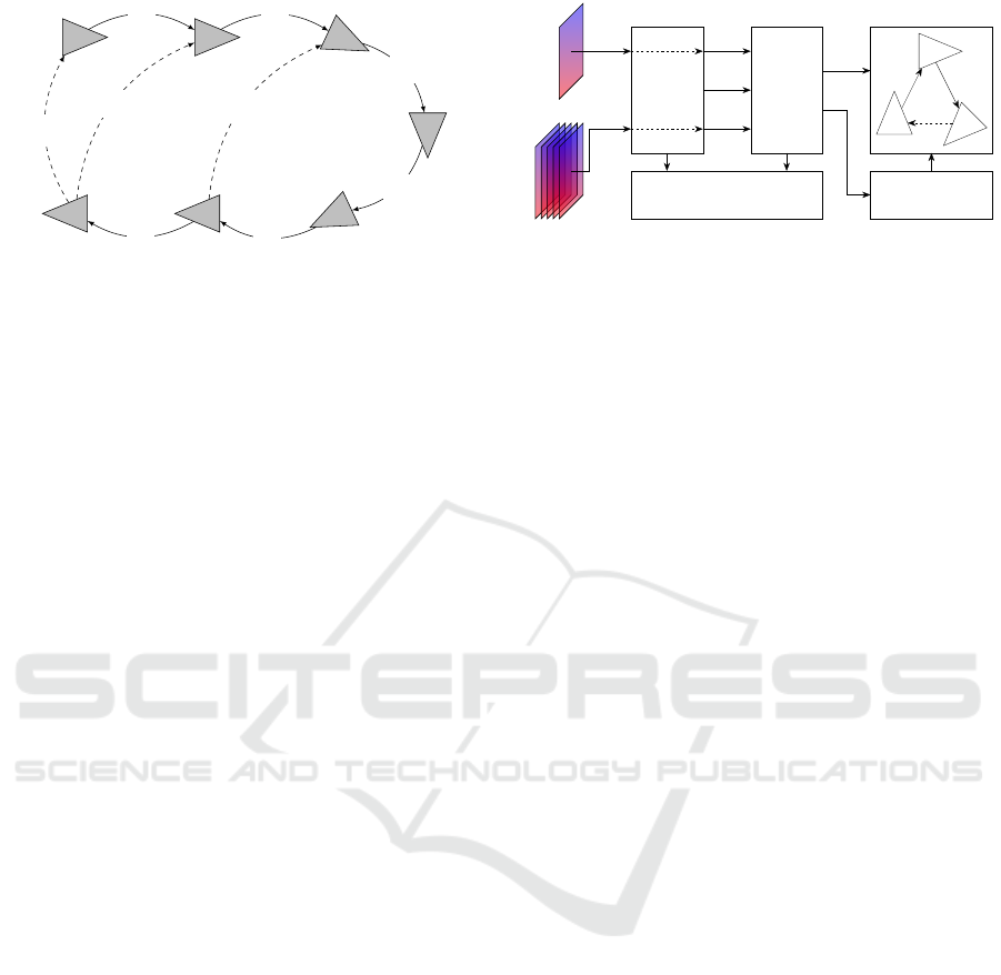
Figure 1: Example of vertices (), odometric edges (→) and
loop closing edges (99K) in a pose graph.
This paper presents a novel approach to per-
form underwater Visual Graph SLAM confronting the
above mentioned problems. To this end, our proposal
combines a traditional approach and a NN to obtain
the best of both worlds. On the one hand, an easily
trainable, lightweight, Siamese NN is used to com-
pare pairs of underwater images and detect loops. On
the other hand, a robust image matcher based on RAn-
dom SAmple Consensus (RANSAC) is used to check
the loops detected by the NN and filter out the wrong
ones without compromising the speed. In this way,
we have the versatility of a lightweight NN as well as
the robustness and accuracy of a traditional method.
By executing these two processes to detect and fil-
ter loops, we are able to feed a Graph SLAM algo-
rithm with clean data, even in underwater environ-
ments, with a huge impact in the final robot pose esti-
mates.
All the annotated and fully commented source
code that we developed in relation to this paper is pub-
licly available. Links to each software repository are
provided throughout the paper.
2 GRAPH SLAM
A pose graph G = {V, E}, illustrated in Figure 1, is
composed of vertices V, which represent robot poses
X
W
i
with respect to an arbitrary, fixed, reference frame
W ; and edges E, which denote relative motions X
i
j
between vertices. In Graph SLAM, odometry is used
to add new vertices and edges; and the detected loops
to create edges between already existing vertices.
A common method to search loops is to compare
each new measurement to all the previous ones. In
visual SLAM this means comparing each new image
to all the previously grabbed images. This can be ex-
tremely time consuming as the number of images in-
creases, thus fast methods to perform the comparison
are desirable. Also, since each new image has to be
independently compared to a large number of past im-
NN
LS
REJECT OPTIMIZER
I
B
I
A
I
A
I
B
LOOP
NO LOOP NO LOOP
LOOP
X
A
B
X
W
B
X
W
C
X
W
A
X
B
C
X
C
A
X
A
B
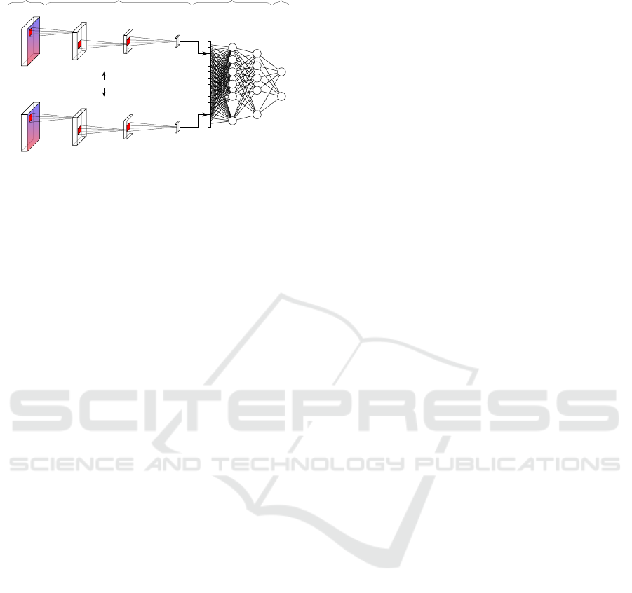
Figure 2: System overview. I
A
and I
B
denote the two input
images.
ages, it is useful to define a method that is potentially
parallelizable. Our proposal is to perform this fast and
potentially parallelizable image comparison by means
of a lightweight NN.
Eventually, the graph is optimized and the vertices
are updated to properly account for the detected loops.
This leads to an improved graph unless the loops are
wrong. Actually, a single wrongly detected loop can
irrevocably corrupt the graph. Given that, in real op-
eration, the number of non-loop situations exceeds by
far the number of loops, even extremely accurate loop
searching methods can result in large numbers of false
positives. Our proposal to solve this problem is to per-
form a Loop Selection (LS) using a robust estimator
based on RANSAC to filter out wrong loops among
those selected by the NN. Since this robust estima-
tor operates on small sets of loops pre-selected by the
NN, the overall speed is not compromised.
By combining a fast loop searching method and a
robust loop rejection algorithm, our proposal ends up
feeding the optimizer with correct sets of loops, as il-
lustrated in Figure 2. Different graph optimization ap-
proaches exist, some of them implicitly dealing with
the false positives (Latif et al., 2014). In this study,
we use a well known implementation of the original
Graph SLAM concepts (Irion, 2019), thus making our
proposal useable with almost any existing graph opti-
mizer.
3 THE NEURAL NETWORK
The NN is in charge of comparing two images and de-
ciding whether they close a loop or not. The proposed
architecture, summarized in Figure 3, is a Siamese
Convolutional Neural Network (CNN) with two main
components, the Global Image Describer (GID) and
the Loop Quantifier (LQ), described next.
VISAPP 2022 - 17th International Conference on Computer Vision Theory and Applications
592

INPUT
LAYER
GLOBAL
IMAGE DESCRIBER
LOOP
QUANTIFIER
OUTPUT
LAYER
64 × 64 × 3
IMAGE B
CONV2D
LKYRELU
BTCHNRM
32 × 32 × 128
CONV2D
LKYRELU
BTCHNRM
16 × 16 × 128
CONV2D
LKYRELU
BTCHNRM
8 × 8 × 16
64 × 64 × 3
IMAGE A
CONV2D
LKYRELU
BTCHNRM
32 × 32 × 128
CONV2D
LKYRELU
BTCHNRM
16 × 16 × 128
CONV2D
LKYRELU
BTCHNRM
8 × 8 × 16
SHARED WEIGHTS
2048
32
16
2
...
...
MERGE
FLATTEN
LD
B
LD
A
Figure 3: The Siamese Neural Network.
3.1 Components
The GID is composed of two Siamese branches, each
one being in charge of processing one image. Be-
ing Siamese they share the same weights and convo-
lutional kernels. The input images are square since
this is a common convention for CNN. To prevent dis-
torted images, our proposal is not to resize the im-
ages provided by the AUV but to crop them using
their shortest dimension as the resulting square side.
The image is then resized to 64×64 pixels using RGB
color encoding. This configuration was experimen-
tally selected though other resolutions and color en-
codings could also be used.
An image is processed by three layers, each one
performing a set of 3×3 convolutions with a stride of
2 using a Leaky Rectifier Linear Unit (ReLU) activa-
tion function with α = 0.2 and a Batch Normalization.
These layers end up providing the so called Learned
Descriptor (LD), which is an 8×8×16 matrix con-
taining essential information about the corresponding
input image. Thus, given two input images, the GID
provides the corresponding learned descriptors LD
A
and LD
B
.
The LQ is in charge of comparing LD
A
and LD
B
to decide if the corresponding images close a loop or
not. To this end, a learnable similarity metric (Mah-
mut Kaya and Hasan Sakir Bilge, 2019) could be
used. Actually, this approach has already succeeded
in performing VLD (Liu et al., 2018). However, these
approaches tend to assume aligned descriptors, which
is not necessarily true in our case. Thus, a different
and more general solution has been adopted.
Our proposal is to flatten and merge LD
A
and LD
B
into a single 1D tensor of size 2048, batch normalize
it, and use it as the input layer of a dense NN in charge
of performing the comparison. The NN has two hid-
den layers with 32 and 16 units each. The output layer
is composed of two units and provides a categorical
output stating if the input images close a loop or not.
This approach is not necessarily symmetric,
meaning that comparing LD
A
and LD
B
may not pro-
duce the same result that comparing LD
B
and LD
A
,
but it does not assumes any alignment between de-
scriptors. Instead, the alignment is learnt during train-
ing.
3.2 Training
Given a sufficiently large dataset, the whole Siamese
NN could be trained. However, in order to reduce the
necessary training data as well as the training time,
our proposal is to proceed in two steps.
During the first step, a Convolutional Auto En-
coder (CAE) is built. A CAE provides an output im-
age that mimics the input image. The input image
goes through two main blocks known as encoder and
decoder. The former transforms the input image into
a latent representation whilst the latter transforms the
latent representation back into the input image. Input
and output being the same, training a CAE is an easy
task since no ground truth is necessary.
Our proposal is to define a CAE using the GID as
encoder, thus the LD being the latent representation.
The decoder is constructed symmetrically to the en-
coder, using transposed convolutions of the appropri-
ate size. In this way, we can easily train the CAE us-
ing solely images of the sea floor. The trained weights
of the encoder can then be used as initial weights for
the GID.
During the second step, the whole NN can be
trained with a dataset with labeled loops. The GID
having properly initialized weights, the training will
be faster and less training data will be necessary. Ac-
tually, the training time and the training set size could
be reduced even more by completely freezing the GID
while in the second training step at the cost of slightly
reducing the overall performance.
An additional advantage of this two step training
is that a trained CAE can be used to provide initial
GID weights for similar environments, thus a library
of GID weights could be constructed in this way.
The complete and fully documented source code
to create and train the GID as part of a CAE
and to create, train and use the the whole Siamese
NN is available at https://github.com/aburguera/
AUTOENCODER and https://github.com/aburguera/
SNNLOOP respectively.
4 LOOP SELECTION
The image pairs that have been classified as loops by
the NN (positives) pass through the Loop Selection
Robust Underwater Visual Graph SLAM using a Simanese Neural Network and Robust Image Matching
593

(LS) to be verified whilst those not classified as loops
(negatives) are discarded. This means that the LS is
aimed at removing false positives but not false nega-
tives. This decision is motivated as follows. On the
one hand, by targeting only the positives the gain in
speed is significant since, as stated previously, their
number is far below the number of negatives in real
Visual SLAM operation. On the other hand, false
positives have a dramatic effect on SLAM operation
whilst false negatives have almost no impact. Thus,
detecting and removing false positives from the equa-
tion is the priority.
Input:
I
A
, I
B
: Input images
K : Number of iterations
M : Number of random samples
N : Minimum consensus size
ε
c
: Maximum correspondence error
Output:
isLoop : True if loop
X
A
B
: Estimated roto-translation
1 ε
A
B
← ∞, isLoop ← False
2 f
A
, d
A
← SIFT (I
A
), f
B
, d
B
← SIFT (I
B
)
3 C ← SIFT MATCH(d
A
, d
B
)
4 for i ← 0 to K − 1 do
5 R ← M random items from C
6 X ← argmin
T
∑
∀(i, j)∈R
||T ⊕ f
A,i
− f
B, j
||
2
7 ε ←
∑
∀(i, j)∈R
||T ⊕ f
A,i
− f
B, j
||
2
8 foreach (i, j) ∈ C − R do
9 if ||X ⊕ f
A,i
− f
B, j
||
2
< ε
c
then
10 R ← R
S
{(i, j)}
11 if |R| > N then
12 X ← argmin
T
∑
∀(i, j)∈R
||T ⊕ f
A,i
− f
B, j
||
2
13 ε ←
∑
∀(i, j)∈R
||T ⊕ f
A,i
− f
B, j
||
2
14 if ε < ε
A
B
then
15 ε
A
B
← E, X
A
B
← X , isLoop ← True
Figure 4: The Loop Selection algorithm.
The LS is summarized in Figure 4, where I
A
and I
B
are two images classified as a loop by the
NN. The algorithm first computes (line 2) the Scale
Invariant Feature Transform (SIFT) features f
i
=
[ f
i,0
, ··· , f
i,Ni
], which are 2D coordinates within the
image f
i, j
= [x
i, j
, y
i, j
]
T
, and the SIFT descriptors d
i
=
[d
i,0
, ··· , d
i,Ni
] of the two images. Afterwards, the de-
scriptors are matched (line 3) and a set C of corre-
spondences is obtained. This set contains the pairs
(i, j) so that d
A,i
matches d
B, j
, which means that f
A,i
and f
B, j
should be corresponding keypoints between
images.
Assuming that the correspondences in C are all
correct, we could compute the roto-translation from
the I
A
to I
B
as the one that minimizes the sum of
squared distances between the corresponding key-
points:
X
A
B
= argmin
X
∑
∀(i, j)∈C
||X ⊕ f
A,i
− f
B, j
||
2
(1)
where ⊕ denotes the composition of transformations
(Smith et al., 1988). It is straightforward to derive a
closed form solution to this Equation from (Lu and
Milios, 1994). However, this is only true if C is cor-
rect, which is not likely to happen since the SIFT
matcher will eventually wrongly detect some corre-
spondences. In particular, if I
A
and I
B
do not close a
loop, no actual correspondences exist and, thus, ev-
erything included in C by the SIFT matcher is wrong.
This means that, in presence of non loop closing im-
ages, an X
A
B
found using Equation 1 would meaning-
less.
Our proposal is to search a sufficiently large sub-
set of C using the RANSAC algorithm so that X
A
B
can be consistently estimated from it. If such sub-
set cannot be found, then the input images do not
close a loop. To this end, a random subset R ∈ C,
called the consensus set, is built (line 5) and the as-
sociated roto-translation X computed (line 6), as well
as the corresponding residual error ε (line 7). After-
wards, each non selected correspondence is individ-
ually tested and included into R if the residual error
it introduces is below a threshold ε
c
(lines 8 to 10).
If the resulting R contains a sufficient number N of
correspondences, then the roto-translation X and the
residual error ε are re-evaluated using the whole R
(lines 11 to 13).
The process is repeated K times and the algorithm
outputs the roto-translation with the smallest residual
error (lines 14 and 15). The key here is that in case of
non-loop closing image pairs the random nature of C
would prevent R to grow up to the required N corre-
spondences. In that case, the algorithm would return
isLoop = False and, so, the input image pair would
be discarded.
As a side effect, the roto-translation X
A
B
corre-
sponding to the best consensus set R is also obtained.
Thus, if the loop is accepted, this roto-translation can
be directly included into the Graph SLAM edge set
E, thus not being necessary to compute it by other
means.
The loop selection source code, together with the
whole Visual Graph SLAM algorithm, is available at
https://github.com/aburguera/GSLAM.
VISAPP 2022 - 17th International Conference on Computer Vision Theory and Applications
594

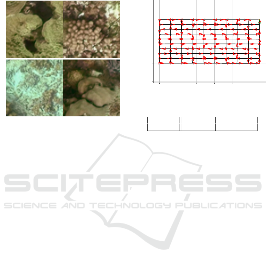
Figure 5: Examples of images used in the experiments.
5 EXPERIMENTS
To validate our proposal, we created four semi-
synthetic datasets named DS1, DS2, DS3 and DS4
by moving a simulated AUV endowed with a bottom
looking camera over two large mosaics, named A and
B, depicting two photo realistic, non overlapping, sea
floors assembled by researchers from Universitat de
Girona (UdG). This semi synthetic approach makes it
possible to have photo realistic underwater images as
well as a perfect, complete, ground truth. The tools
we developed to build these datasets are available at
https://github.com/aburguera/UCAMGEN. Figure 5
shows some examples of the images in the datasets.
DS1 and DS2 were constructed by defining a grid
over mosaics A and B respectively, placing the simu-
lated AUV at the center of each grid cell with a ran-
dom orientation and then making it perform a full
360
o
rotation and grabbing an image every 10
o
. These
datasets, which provide an extensive view of the envi-
ronment with a wide range of AUV orientations, are
composed of 35640 (DS1) and 14850 (DS2) images.
DS3 and DS4 were built by making the AUV grab
images while performing a sweeping trajectory over
mosaics A and B respectively. Figure 6 shows the
trajectory in DS4. These datasets, which represent a
realistic AUV mission, are composed of 15495 (DS3)
and 6659 (DS4) images. They also contain dead reck-
oning information and the ground truth AUV poses
and loop information among others.
It is important to emphasize that, given that mo-
saics A and B do not overlap at all, DS1 and DS2 are
completely disjoint, as well as DS3 and DS4.
0 5 10 15 20 25
m
− 5
0
5
10
15
m
Figure 6: The AUV trajectory.
Table 1: Siamese NN evaluation.
A 0.966 P 0.950 R 0.983
F 0.051 F1 0.966 AUC 0.992
5.1 Neural Network Evaluation
Following the method described in Section 3.2, we
first trained the CAE using DS1, randomly shuffling
the images at each epoch. Afterwards, we used DS2
to evaluate the CAE. The trained CAE was able to
reconstruct the images in DS2 almost perfectly with a
Mean Absolute Error (MAE) of 0.00425 and a Mean
Square Error (MSE) of 0.00003. The CAE encoder
weights were used as the initial GID weights in the
subsequent training.
The whole Siamese NN was trained using DS3. At
each training epoch, a balanced subset (i.e. having the
same number of loops and non loops) of DS3 was ran-
domly selected and the resulting data shuffled. After
training, the Siamese NN was evaluated using a bal-
anced version of DS4. The evaluation results in terms
of accuracy (A), precision (P), recall (R), fall-out (F),
F1-Score (F1) and area under the Receiver Operating
Characteristic (ROC) curve (AUC) are shown in Ta-
ble 1. As it can be observed, we achieved very high
quality metrics, surpassing the 99% of AUC and hav-
ing a fall-out close to the 5% meaning that the NN
is really good not only at detecting loops but also at
discarding non loops.
5.2 LS Evaluation
The LS has been evaluated as part of a full Visual
Graph SLAM system using DS4 (thus, the AUV per-
forming the trajectory shown in Figure 6) and the
graph optimizer in (Irion, 2019). To reduce the com-
putational burden, the comparison between each new
image and the previous ones is performed in steps of
Robust Underwater Visual Graph SLAM using a Simanese Neural Network and Robust Image Matching
595

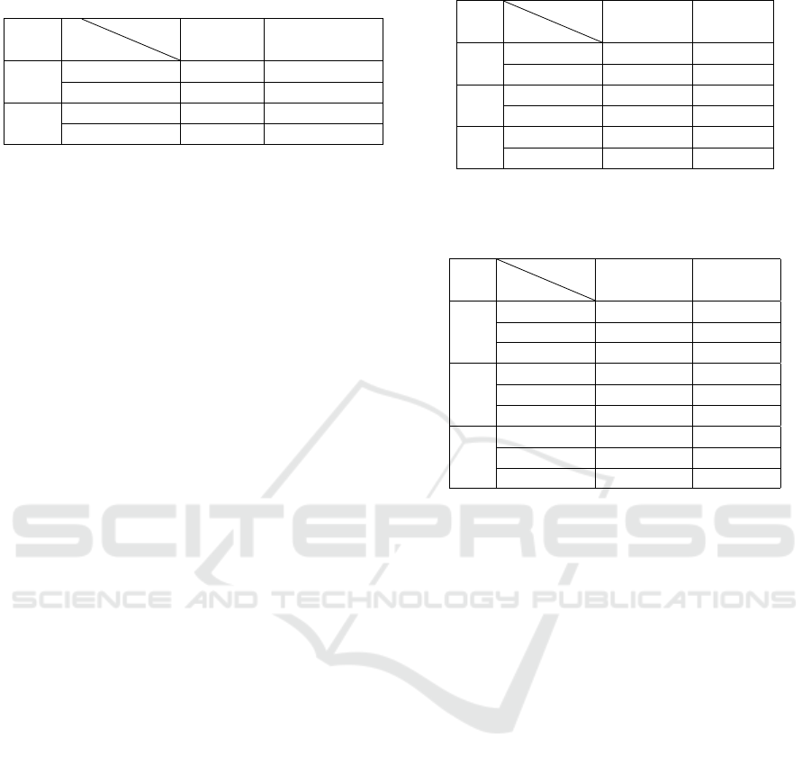
Table 2: Confusion matrix showing actual (ACT) vs pre-
dicted (PRED) loops.
LS
ACT.
PRED.
LOOP NON-LOOP
NO
LOOP 2130 TP 3227 FN
NON-LOOP 5505 FP 184159 TN
YES
LOOP 1353 TP 4004 FN
NON-LOOP 0 FP 189664 TN
five. The X
A
B
computed by LS is used to create the
edges representing the motion between loop closing
images.
As a baseline, we reproduced the same process but
disabling the LS, thus the NN being the sole loop de-
tector. Since the NN has already been evaluated, this
will help us in assessing the benefits of LS. To pro-
vide a fair comparison, even though LS is not used to
filter loops, it is to compute the required X
A
B
. If LS
cannot provide a motion estimate, Equation 1 using
all the correspondences in C is used instead.
Table 2 summarizes the obtained results. Us-
ing the confusion matrix we obtain a baseline accu-
racy and fall-out of 0.955 and 0.029, which are sim-
ilar to those obtained when evaluating the NN with
a balanced dataset. The baseline precision (0.278),
recall (0.397) and the F1-Score (0.164), however,
are far below those previously obtained. Moreover,
the baseline results even show more false positives
(5505) than true positives (2130). This is due to
the extremely unbalanced data when searching loops
through a realistic mission: only 5357 of the tested
image pairs were actually loops in front of 189664
non loops.
Our proposal, the LS, has rejected a total of 6282
image pairs that were classified as loops by the NN.
Among them, 5505 were correctly rejected and 777
incorrectly rejected. Taking into account that, because
of that, the resulting number of false positives is 0, we
can conclude that LS is a good approach to help in
detecting loops in a Visual Graph SLAM context.
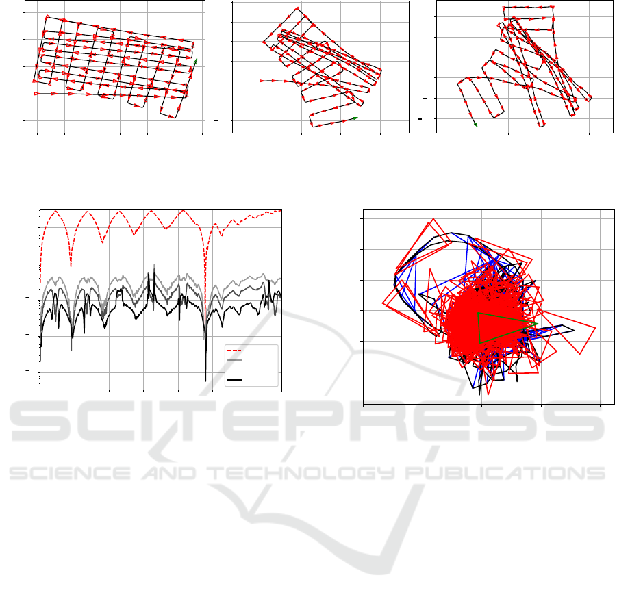
5.3 Visual SLAM Evaluation
To evaluate the whole Visual Graph SLAM approach,
we corrupted the dead reckoning estimates in DS4
with three different noise levels (NL) as shown in Fig-
ure 7. In this way, we can observe how our proposal
behaves in front of good and bad dead reckoning. For
each NL we performed Visual Graph SLAM with the
LS disabled and enabled as described in Section 5.2.
This results in six different configurations.
As a quality metric, we computed the Absolute
Trajectory Error (ATE), which is a vector contain-
ing the distances between each estimated graph ver-
Table 3: Absolute Trajectory Error.
NL
ATE
LS
NO YES
1
µ 15.689 m 0.071 m
σ 7.459 m 0.052 m
2
µ 15.619 m 0.139 m
σ 7.444 m 0.068 m
3
µ 15.684 m 0.287 m
σ 7.440 m 0.123 m
Table 4: Average time per tested image pair consumed by
the NN, the LS and the graph optimizer (OPT). N.A. means
Not Applicable.
NL
TIME
LS
NO YES
1
NN 0.484 ms 0.499 ms
LS N.A. 1.472 ms
OPT 30.857 ms 1.499 ms
2
NN 0.482 ms 0.458 ms
LS N.A. 1.413 ms
OPT 30.729 ms 1.605 ms
3
NN 0.487 ms 0.460 ms
LS N.A. 1.413 ms
OPT 30.036 ms 1.647 ms
tex and the corresponding ground truth (Ceriani et al.,
2009). Figure 8 shows, in logarithmic scale, the ATE
for the three noise levels when using LS compared to
the ATE for noise level 1 when LS is not used. Table
3 shows the mean µ and the standard deviation σ of
the ATE for the six the mentioned configurations.
As it can be observed, not using LS results in ex-
tremely large errors that are almost removed when en-
abling LS. For example, whereas the mean ATE al-
ways surpasses the 15 m, it is below the 10 cm for
NL=1 and below the 30 cm when NL=3. The standard
deviation is also significantly smaller when using LS,
meaning that LS provides stability to the system.
It can also be observed how the ATE increases
with the noise level when LS is enabled, going from
µ=0.071 m when NL=1 to µ=0.287 m when NL=3.
This is reasonable, since the odometric error influ-
ences the estimated vertex poses. However, this trend
does not appear when LS is disabled, the ATE being
almost the same (µ '15.6 m, σ ' 7.4) for all noise
levels. This is because the resulting trajectory is so
bad due to the false positives that the odometric noise
has almost no influence in it.
The time consumption has also been measured ex-
ecuting the provided Python implementation over an
Ubuntu 20 machine with an i7 CPU at 2.6 GHz. Ta-
ble 4 shows the average time per compared image
pair spent by the NN, the LS (when applicable) and
by the graph optimizer. The most relevant conclusion
VISAPP 2022 - 17th International Conference on Computer Vision Theory and Applications
596

0 5 10 15 20 25 30
m
− 5
0
5
10
15
m
0 1 0 20 3 0
m
10
5
0
5
10
15
20
m
0 10 20 30
m
10
5
0
5
10
15
m
(a) (b) (c)
Figure 7: Trajectory corrupted with (a) Noise level 1. (b) Noise level 2. (c) Noise level 3.
0 200 400 600 800 1000 1200 1400
Graph vertex
10
3
10
2
10
1
10
0
10
1
ATE (m )
NO LS
LS,NL= 3
LS,NL= 2
LS,NL= 1
Figure 8: Absolute Trajectory Error using LS (showing the
three noise levels) and not using LS (only noise level 1) in
logarithmic scale.
that arises from this time measurements is that using
LS leads to an overall huge improvement: the wrong
loops make the optimization process so slow that even
considering the time spent by LS, using LS is ex-
tremely faster in average. For example, whereas not
using LS requires more than 30 ms per compared im-
age pair, using LS reduces this average time to about
3.5 ms in total. It is also remarkable the speed of the
NN, being the smallest in all cases. Also, it is no sur-
prise that the time spent by the NN does not depend
on the noise level.
Figure 9 depicts the obtained graph for NL=3
when LS is not enabled. Results for other noise level
are similar. It can be observed how the existing false
positives lead the graph optimizer to a state which has
no ressemblance to the expected trajectory.
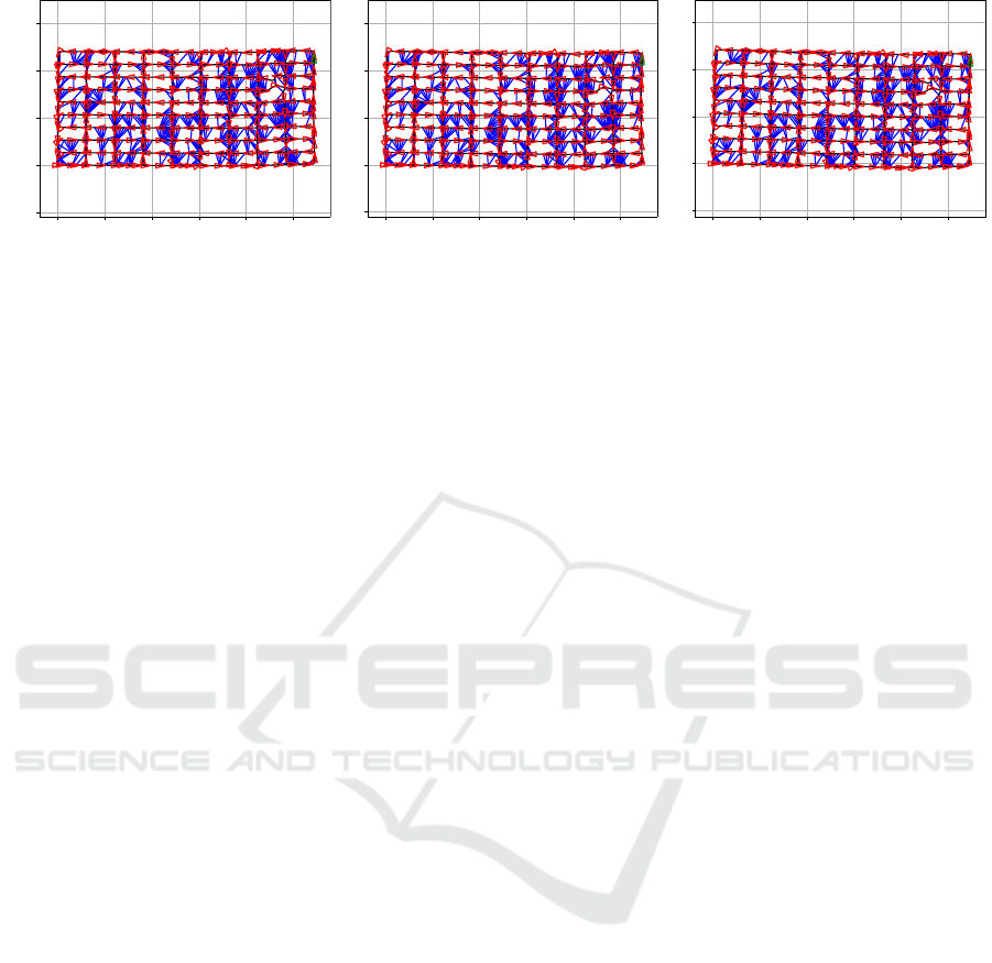
Figure 10 shows the resulting trajectories when
using LS to remove false positives for the three noise
levels. The three trajectories are almost identical to
the ground truth (Figure 6) independently of the odo-
metric error (Figure 7) and in spite of the reduction in
the number of true positives. It becomes clear, thus,
that removing false positives is far more imporant that
preserving true positives.
− 2 − 1 0 1 2
m
− 1 .0
− 0 .5
0.0
0.5
1.0
1.5
2.0
m
Figure 9: Resulting trajectory with NL=3 when LS is not
used. The triangles represent the AUV orientation at some
points and blue lines denote the detected loops.
6 CONCLUSION
One of the major challenges associated with Visual
Graph SLAM arises because wrongly detected loops
heavily degrade the underlying graph. Since the
amount of non loop closing image pairs is much larger
than the amount of loop closing image pairs, the num-
ber of wrongly detected loops can easily surpass the
amount of those properly detected. Having a robust
method to detect and remove wrong loops is, thus,
crucial.
Our proposal takes advantage of the speed and
versatility of a small, lightweight, Siamese NN and
the accuracy and robustness of RANSAC. At each
time step, the most recent image grabbed by the AUV
is compared to the previous ones using the NN. Those
pairs discarded by the NN are not included into the
graph. Those that are accepted go through a second,
exhaustive, test using RANSAC. Using this approach,
we achieve not only a robust but also a fast method to
feed any Visual Graph SLAM algorithm with clean
loop information.
Robust Underwater Visual Graph SLAM using a Simanese Neural Network and Robust Image Matching
597

0 5 10 15 2 0 2 5
m
− 5
0
5
10
15
m
0 5 10 15 20 25
m
− 5
0
5
10
15
m
0 5 10 15 20 2 5
m
− 5
0
5
10
15
m
(a) (b) (c)
Figure 10: Resulting trajectories with LS enabled using (a) noise level 1, (b) noise level 2 and (c) noise level 3. The triangles
represent the AUV orientation at some points and blue lines denote the detected loops.
During the experiments, the NN performed
195021 image comparisons spending, in average, less
than 0.5 ms per image pair. Only 5505 of the com-
pared image pairs were false positives. Even though
this is less than a 3%, they lead to more than 15 m of
mean ATE. Thanks to the LS, however, the number
of false positives was reduced to zero and the ATE to
values between 7.1 cm and 29.7 cm. By executing LS
only with the pairs classified as positives by the NN
the gain in speed is considerable.
Overall, our proposal is able to robust and fastly
search loops, being able to produce high quality Vi-
sual Graph SLAM algorithms even in front of large
odometric noise in underwater scenarios.
ACKNOWLEDGEMENTS
Grant PID2020-115332RB-C33 funded by MCIN /
AEI / 10.13039/501100011033 and, as appropriate,
by ”ERDF A way of making Europe”.
REFERENCES
Arshad, S. and Kim, G. W. (2021). Role of deep learning in
loop closure detection for visual and lidar SLAM: A
survey. Sensors (Switzerland), 21(4):1–17.
Bonin-Font, F., Burguera, A., and Oliver, G. (2013). New
solutions in underwater imaging and vision systems.
In Imaging Marine Life: Macrophotography and Mi-
croscopy Approaches for Marine Biology, pages 23–
47.
Burguera, A. and Bonin-Font, F. (2020). Towards visual
loop detection in underwater robotics using a deep
neural network. Proceedings of VISAPP, 5:667–673.
Ceriani, S., Fontana, G., Giusti, A., Marzorati, D., Mat-
teucci, M., Migliore, D., Rizzi, D., Sorrenti, D. G.,
and Taddei, P. (2009). Rawseeds ground truth collec-
tion systems for indoor self-localization and mapping.
Autonomous Robots, 27(4):353–371.
Irion, J. (2019). Python GraphSLAM. Available at: https:
//github.com/JeffLIrion/python-graphslam.
Latif, Y., Cadena, C., and Neira, J. (2014). Robust graph
SLAM back-ends: A comparative analysis. Proceed-
ings of IEEE/RSJ IROS, (3):2683–2690.
Liu, H., Zhao, C., Huang, W., and Shi, W. (2018). An
End-To-End Siamese Convolutional Neural Network
for Loop Closure Detection in Visual Slam System. In
Proceedings of the IEEE ICASSP, pages 3121–3125.
Lowry, S., Sunderhauf, N., Newman, P., Leonard, J. J.,
Cox, D., Corke, P., and Milford, M. J. (2016). Vi-
sual Place Recognition: A Survey. IEEE Transactions
on Robotics, 32(1):1–19.
Lu, F. and Milios, E. E. (1994). Robot pose estimation in
unknown environments by matching 2D range scans.
Proceedings of the IEEE Computer Society Confer-
ence on Computer Vision and Pattern Recognition,
pages 935–938.
Mahmut Kaya and Hasan Sakir Bilge (2019). Deep Metric
Learning : A Survey. Symmetry, 11.9:1066.
Merril, N. and Huang, G. (2018). Lightweight Unsuper-
vised Deep Loop Closure. In Robotics: Science and
Systems.
Smith, R., Self, M., and Cheeseman, P. (1988). A stochas-
tic map for uncertain spatial relationships. Proceed-
ings of the 4th international symposium on Robotics
Research, (0262022729):467–474.
Thrun, S. and Montemerlo, M. (2006). The graph SLAM
algorithm with applications to large-scale mapping of
urban structures. International Journal of Robotics
Research, 25(5-6):403–429.
VISAPP 2022 - 17th International Conference on Computer Vision Theory and Applications
598