An Initial Study in Wood Tomographic Image Classiﬁcation using the

SVM and CNN Techniques

Antonio Alberto Pereira Junior

and Marco Antonio Garcia de Carvalho

School of Technology, University of Campinas, R. Paschoal Marmo 1888, Limeira/SP, Brazil

Keywords:

Ultrasound Tomography, Wood Internal Pathologies, Image Interpolation, Data Augmentation, Classiﬁcation.

Abstract:

The internal analysis of wood logs is an essential task in the ﬁeld of forest assessment. To assist in the

identiﬁcation of anomalies within wood logs, methods from the Non-Destructive Testing area can be used, as

the acoustic methods. The ultrasound tomography is an acoustic method that allows to evaluate the internal

conditions of wood logs, through the analysis of wave propagation, without being necessary to cause damage

to the specimen. The images generated by ultrasound tomography can be improved by spatial interpolation,

i.e., estimating the values of wave propagation not measured in the initial examination. In this paper we

present an initial study of classiﬁcation techniques in order to identify tomographic images with anomalies.

In our approach we consider three different classiﬁers: k-Nearest-Neighbor (k-NN), Support Vector Machine

(SVM) and Convolutional Neural Network (CNN). Experiments were conducted comparing them by means

of metrics obtained from the confusion matrix. We build a dataset with 5000 images using data augmentation

process. The quantitative metrics demonstrate the effectiveness of CNN when compared with k-NN and SVM

classiﬁers.

1 INTRODUCTION

Non-Destructive Tests (NDTs) are studied as they al-

low the evaluation of the specimen while maintaining

its integrity. In woods, the use of non-destructive test-

ing is interesting because it allows to decide which

information is needed to characterize each wood and

to know how to use the information to explain the be-

havior of the wood (Bucur, 2006).

One of the most used NDT technique is the ul-

trasound tomography. The ultrasound tomography al-

low the evaluation of the internal condition in woods

by measuring the propagation time of the ultrasonic

pulse, which does not cause any damage to the ob-

ject. Usually, the images obtained by the ultrasound

tomography don’t describe exactly the image regions

associated with the anomaly. For this reason, the pres-

ence of an expert is necessary to identify an exact re-

gion of the defect based on the tomography image. A

strategy used in order to improve the quality of gen-

erated images by ultrasound tomography is data in-

terpolation. Some of the main techniques are Inverse

Distance Weighting (Shepard, 1968), Ellipse Based

https://orcid.org/0000-0002-2304-3068

https://orcid.org/0000-0002-1941-6036

Spatial Interpolation (Du et al., 2015), and Path Con-

textual Analysis (Strobel, 2017).

Alternatively to the visual analysis of tomographic

images, there is an increase in the use of digital im-

age processing techniques and data classiﬁcation (Du

et al., 2019)(Mu et al., 2015). However, there are still

few works in the literature that address the classiﬁca-

tion of image regions in wood logs.

The goal of this paper is to propose a classiﬁca-

tion approach in order to identify images with de-

fects in woods from the images generated by ultra-

sound tomography. To achieve this goal, we accom-

plish an initial study using three different techniques:

k-Nearest-Neighbor (k-NN), Support Vector Machine

(SVM) and Convolutional Neural Network (CNN).

The main contributions of this initial study are: (i)

enable the use of CNN using a dataset with few im-

ages and obtained with data augmentation support;

(ii) compare different image classiﬁcation strategies.

Therefore, this work compares the classiﬁcation tech-

niques by means of metrics calculated from a confu-

sion matrix. Also, as a secondary objective, this work

intends to gather data from ultrasound experiments on

wooden logs to generate a dataset and make it pub-

licly available.

Pereira Junior, A. and Garcia de Carvalho, M.

An Initial Study in Wood Tomographic Image Classiﬁcation using the SVM and CNN Techniques.

DOI: 10.5220/0010881700003124

In Proceedings of the 17th International Joint Conference on Computer Vision, Imaging and Computer Graphics Theory and Applications (VISIGRAPP 2022) - Volume 4: VISAPP, pages

575-581

ISBN: 978-989-758-555-5; ISSN: 2184-4321

575

The reminder of this paper is organized as follows:

In Section 2 we address some related works and ba-

sic concepts. We describe how a tomographic image

is obtained by means of an ultrasound inspection test.

A description of our proposed method is addressed in

Section 3. We present brieﬂy each one of the classiﬁ-

cation techniques used in this work. The experiments

and results are shown in Section 4. Finally, in Section

5 we presented our conclusions.

2 BACKGROUND AND RELATED

WORKS

In this section we introduce basics concepts of ultra-

sound tomography on woods, as well as we brieﬂy de-

scribe data interpolation techniques used in this work.

Finally, some related works on wood classiﬁcation are

presented.

2.1 Concepts of Ultrasound

Tomography

Tomography is an acoustic non-destructive technique

used to analyze the structure and composition of ob-

jects (Grangeat, 2010). The ultrasound tomography

allows to evaluate the internal conditions of wood logs

by means of an ultrasound test, illustrated in Figure 1.

Figure 1: Ultrasound test on wood logs. The yellow arrows

show the transducers used to measure the wave propagation

time. SOURCE: Adapted from (Secco, 2011).

The ultrasound test measures the wave propaga-

tion time in the wooden logs, known as Time Of Flight

(TOF). Therefore, the acoustic velocity can be deter-

mined as the distance between the transducers (path

length) is also known.

In addition, the ultrasound test is performed ac-

cording to a wood representation scheme, which

provides a guide for positioning the transducers.

The main existing schemes, or inspection grids, are

diffraction and straight grids(Secco, 2011). The in-

spection grids deﬁne routes or paths through which

wave propagation occurs and are important attributes

in the generation of tomographic images.

2.2 Interpolation and Image Creation

In this work, spatial interpolation will be used to es-

timate the acoustic velocity values of points that do

not belong to a diffraction grid route. We select two

different methods in order to interpolate the data: the

Inverse Distance Weighting and the Path Contextual

Analysis.

Inverse Distance Weighting - IDW

The IDW interpolation technique is simple and com-

putationally efﬁcient. The value of a point to be inter-

polated is given by the weighted average of the known

values of its neighborhood (Shepard, 1968). In this

case, the weight refers to the distance between the

points.

Path Contextual Analysis

In this method, the interpolation is accomplished ac-

cording to the position of the unknown point, consid-

ering two different regions to be analyzed: near to the

bark and to the pith wood(Strobel, 2017). The Path

Contextual Analysis uses an Ellipse Based Spatial In-

terpolation Algorithm in order to estimate the velocity

values in unknown grid cells that represent unknown

points(Du et al., 2015). In this method it is considered

that the propagation of the ultrasonic pulse has an el-

liptical inﬂuence zone around the route generated by

the positioning of the transducers.

2.3 Related Works

There are several works related to the application of

ultrasound tomography in woods. Usually, the works

intends to solve problems regarding to the generation

of images through ultrasound tomography, improve-

ment of interpolation methods and evaluation of to-

mographic image quality.

The works related to the investigation of the ultra-

sound tomography in wood seeks to understand the

relationships between: the coupling of transducers in

wood, problems related to the anisotropy, signal at-

tenuation, number of measurement points, frequency

used in the test, arrangements or meshes for testing

and type of transducers ((Socco et al., 2004), (Bucur,

2005),(Lin et al., 2008),(Palma et al., 2018)).

There are works which the authors report the use

of algorithms to reconstruct the internal characteris-

tics of the woods. For those studies, spatial interpola-

tion algorithms are studied. In (Zeng et al., ) is pre-

sented an approach using affected areas through an

ellipse with the same eccentricity. This method is im-

proved by the authors (Du et al., 2015) considering

VISAPP 2022 - 17th International Conference on Computer Vision Theory and Applications

576

ellipses with different eccentricities, giving rise to the

Ellipse Based Spatial Interpolation (EBSI) method.

Finally, (Du et al., 2018) and (Du et al., 2019) present

some improvements to the EBSI method. As a way

of evaluating wood considering different axis, the au-

thor (Feng et al., 2018) performs an experiment with

the Radial and Longitudinal axis, and also proposes

the interpolation method Velocity Correction Interpo-

lation(VCI).

In general, methods are not quantitatively evalu-

ated in order to verify tomographic image quality. In

(Strobel et al., 2018) is presented a quantitative eval-

uation approach, using the confusion matrix, compar-

ing the tomography image with a ground-truth image.

There are also works that use artiﬁcial intelli-

gence (AI) methods to identify defects in wood (Zhu

et al., 2009), (Mu et al., 2015), and to reconstruct

the internal characteristics of wood (Effendi et al.,

2019),(Hansson et al., 2015). However, in these

works other inspection techniques are considered,

such as CT and X-Ray.

There’s an alternative for the reconstruction of to-

mography images using the technique of deep learn-

ing and contour constraint (DLCC) (Du et al., 2019).

In these work the deep learning algorithm was applied

to detect the size, texture and limit the contour of de-

fects in the wood.

Studies on ultrasound tomography are taking ad-

vantage of AI concepts as a tool to identify defects in

wood. However, there are opportunities to be devel-

oped, due to the low amount of works that approach

these techniques. In order to cover this gap, this work

intends to implement classiﬁcation techniques for the

identiﬁcation of tomographic images of wood logs

with defects.

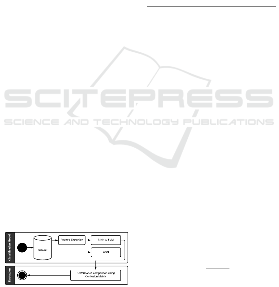
3 PROPOSED APPROACH

This section discuss the approach proposed in this pa-

per. The workﬂow shown in the Figure 2 illustrates

a general view of each step of our work: (i) image

acquisition; (ii) feature extraction; (iii) classiﬁcation

using k-NN, SVM and CNN; and (iv) performance

evaluation.

Classification Model

Evaluation

Dataset

Feature Extraction

CNN

k-NN & SVM

Performance comparison using

Confusion Matrix

Figure 2: Workﬂow of the proposed approach.

The following subsections explain each step of our

proposed approach.

3.1 Dataset and Evaluation Protocol

The image were obtained from the Non-Destructive

Laboratory (LabEND) of the University of Campinas

- UNICAMP. Table 1 show the wood species and pro-

vides a brief description of the wood logs used in this

work.

Table 1: Wood logs used in the experiments. SOURCE:

(Strobel, 2017).

Species Description

Lonchocarpus It has artiﬁcial circular hollows 5cm

in diameter.

Liquidambar styraci-

ﬂua

Small area with an early stage of

fungal decomposition near to the

pith, plus lateral cracks from pith to

bark.

Platanus sp Most of the wood shows signs of

fungus attacks and there are some

empty areas caused by termites.

Centrolobium sp Contains central hollow due to ter-

mite attack.

Due to the limited amount of images, a process of

data augmentations is also required to be able to in-

crease the size and the quality of data (Shorten and

Khoshgoftaar, 2019). This process consists of manip-

ulating an existing image by submitting it to geomet-

ric transformations, i.e., rotation and resizing. The ad-

dition of noise is another technique used to increase

the amount of images, one of the most known tech-

niques is the interference of Salt & Pepper, which

consists of adding white and black pixels in a sparse

occurrence. Labelling is the last step to create the

dataset.

First, it’s necessary to determine an area in the

ultrasound tomography image and associate to the

“anomaly” class. An initial labeling process had been

done in previous work (Strobel, 2017) and served as

the reference for the dataset annotation.

Finally, three metrics were employed to evaluate

the performance of the classiﬁcation technique, com-

paring its results with the ground-truth provided by

the labelling process: (1) recall - R; (2) precision - P;

and (3) accuracy - Acc. The equations are deﬁned as

follows:

R =

T P

T P + FP

(1)

P =

T P

T P + FN

(2)

Acc =

T P + T N

T P + T N + FP + FN

(3)

An Initial Study in Wood Tomographic Image Classiﬁcation using the SVM and CNN Techniques

577

where TP, TN, FP and FN represents, respectively,

true-positive, true-negative, false-positive, and false-

negative values.

3.2 Feature Extraction

The purpose of this step is to obtain descriptors that

are able to represent the texture characteristics of the

tomographic image. The following subsections de-

scribes the texture descriptor we use in this work: the

Gray Levels Co-occurrence Matrix (GLCM) and the

Local Binary Pattern (LBP).

3.2.1 Gray Levels Co-occurrence Matrix

Gray Level Co-occurrence Matrix (GLCM) is a

method of extracting texture features from grayscale

image (Robert et al., 1973). Through each vec-

tor of characteristics obtained, another 14 charac-

teristics can be obtained from the generated matrix,

among them: Mean, Variance, Entropy, Dissimilarity,

Contrast, Homogeneity, Correlation, Energy, Clus-

ter Shade, Cluster Prominence, Sum Entropy, Sum

Mean, Entropy Difference, Sum Variance.

3.2.2 Local Binary Pattern

Local Binary Pattern (LBP) is a method to describe

the local image pattern (Ojala et al., 1996). LBP

assumes that textures can be described by measure-

ments: local spatial patterns and gray level contrast.

This method extracts local texture information and

sets a threshold for a number of neighbors, in the

value of the central pixel in that deﬁned local neigh-

borhood.

3.3 Classiﬁcation Techniques

Classiﬁcation techniques are use to classify datasets

with known deﬁnitions of groups. In this case it’s

presented to the model samples of desired inputs and

outputs, previous deﬁned by an human. The goal of

this technique is to learn a general rule that map the

inputs and outputs to the overall model.

This work intends to detect the region of the im-

age that has the anomaly. Therefore, classiﬁcations

models will be used to execute this proposal. We

use two supervised algorithms: k-Nearest-Neighbor

(k-NN) and Support Vector Machines (SVM). Those

two algorithms was chosen due to common use in the

classiﬁcation tasks. Additionally, as a tentative to im-

prove the classiﬁcation performance, a Convolutional

Neural Network (CNN) model is also applied in this

work. By the end, we should be able to compare both

models and then determine which one is the best to

identify anomaly in woods. The following subsection

describes each one of the classiﬁcation techniques.

3.3.1 k-NN

The k-Nearest-Neighbor (k-NN) (Cover and Hart,

1967) is also known as lazy learn or instance-based,

which means that the algorithm does not perform the

model deﬁnition or generalization when training data

is received, but during execution time. This analogi-

cal learning technique performs peer-to-peer compar-

isons to identify similarities between input data. To

determine which data are closest or similar, it is nec-

essary to describe them using distance notation, i.e.,

the euclidean distance.

3.3.2 Support Vector Machine

The Support Vector Machines (SVM) (Suykens and

Vandewalle, 1999) is a classiﬁcation technique that

can be applied to linearly separable or non-linearly

separable data. This technique aims to determine the

best hyperplane for class segregation using vectors to

support this determination. In this work, we use dif-

ferent kernels to see the performance of each one sep-

arately.

3.3.3 Convolutional Neural Network

The Convolutional Neural Network (CCN) is one of

the most popular deep neural network. This network

can have multiple layer, in particular: the convolu-

tion layer, ReLU, pooling layer and fully connected

layer (Albawi et al., 2017). The CNN have the ability

to train large datasets and considers millions of pa-

rameters, because of that, this network is commonly

used in area of image recognition, object detection

and computer vision.

A CNN performs automatically the step of fea-

ture extraction by using the convolution layer. So

the model can learn all features in one pass instead

of having the features being selected by an engineer.

For those aspects, a Convolutional Neural Network

model is going to be used in this work to avoid the

features extraction step. In contrast, the need for a

large amount of training data is an important feature

of CNNs. In order to mitigate this requirement, we

apply data augmentation techniques in our dataset.

The Convolutional Neural Network that will be used

in this work is the SDD MobileNetV2 (Sandler et al.,

2018). This Convolution Neural Network is available

in Tensorﬂow 2 (Abadi et al., 2015) which uses the

object detection approach to detect bounding boxes.

This model was chosen due to the speed and to the in-

put size of tomography image available in the dataset.

VISAPP 2022 - 17th International Conference on Computer Vision Theory and Applications

578

4 EXPERIMENTS AND INITIAL

RESULTS

This section presents the conducted experiments re-

garding the initial study of different classiﬁcation

techniques to assess the tomographic images. All

experiments are performed using an Intel i5 desk-

top, 16GB RAM running macOS 10.15 Catalina.

Our computational implementation was developed

in Python 3.0 using Google Colaboratory (Bisong,

2019). We present the results and compare the per-

formance of the techniques with each other.

As mentioned before, a data augmentation process

was used to build the entire dataset. At the end of

this process, the dataset had 5000 tomographic im-

ages and the annotation ﬁles related to them.

The ﬁrst step for the common supervised models

is to extract the vector of features from each tomo-

graphic image. To be able to extract those feature

vectors it was necessary to get the features that be-

longs to the anomaly and the features that correspond

to the healthy wood region. Those vectors generated

by the feature extraction are the input for the classiﬁ-

cation models: SVM and k-NN. The dataset was split

in 70% of images for training and 30% for test step.

Our ﬁrst experiment concerns studying different

types of SVM usage conﬁgurations. Table 2 shows

the results of the SVM model using different types of

Kernel. We evaluate the performance of the classi-

ﬁcation task under the different metrics described in

the section 3.1. The best performance for each metric

are highlighted in bold.

Table 2: Effectiveness of the SVM technique using different

combinations (in bold, the highest value observed in each

column).

SVM (Kernel) - Feature Accuracy Recall Precision

SVM (Linear) - LBP 76.00 87.80 73.46

SVM (Linear) - GLCM 74.66 88.09 72.54

SVM (Polynomial) - LBP 85.33 92.68 82.60

SVM (Polynomial) - GLCM 68.00 64.28 75.00

SVM (RBF) - LBP 86.66 95.12 82.97

SVM (RBF) - GLCM 81.33 88.09 80.43

SVM (Sigmoid) - LBP 64.00 60.97 69.44

SVM (Sigmoid) - GLCM 64.00 66.66 68.29

According to Table 2, the best result of Accuracy,

Recall and Precision occurred using the SVM with the

Kernel RBF and the LBP feature. The second exper-

iment analyzes the use of the k-NN classiﬁer. Table

3 shows the results of the k-NN model. The values

of k was chosen based on a experiment with a small

portion of the dataset. This experiment showed lim-

ited improvements in the accuracy when k was incre-

mented with a values less than 50 for each run. For

this reason the experiment showing in the table be-

low for the classiﬁer k-NN is going to consider k=50,

k=100, and k=150.

Table 3: Effectiveness of the k-NN technique using different

combinations (in bold, the highest value observed in each

column).

k-NN (k=Value) - Feature Accuracy Recall Precision

k-NN (k=50) - LBP 78.66 85.36 77.77

k-NN (k=50) - GLCM 74.66 76.19 78.04

k-NN (k=100) - LBP 74.66 80.48 75.00

k-NN (k=100) - GLCM 54.66 45.23 66.33

k-NN (k=150) - LBP 57.33 43.90 66.66

k-NN (k=150) - GLCM 49.33 16.66 70.00

In the case of the k-NN classiﬁer, the best result

was the one that use LBP considering k=50. Over-

all, the results shown in Tables 2 and 3 presents good

accuracy values, especially those using LBP descrip-

tor. The last classiﬁcation method addressed in this

work was the CNN. In this case, our experiment con-

sists of comparing the best performances of SVM and

k-NN, using LBP texture descriptor, with the results

obtained by using the CNN SDD MobileNetV2. Ta-

ble 4 shows the results.

Table 4: Performance comparison (in bold, the highest

value observed in each column).

Technique Accuracy Recall Precision

SVM (RBF) - LBP 86.66 95.12 82.97

k-NN (k=50) - LBP 78.66 85.36 77.77

SDDMobileNetV2 89.00 93.40 97.30

As we can observe in Table 4, the performance of

the SDDMobileNetV2 classiﬁer was better than that

obtained by the other classiﬁers, regardless the used

metric, Accuracy, Recall or Precision. Nevertheless,

the three ﬁrst experiments concerns to the task of clas-

sify the entire image as having or not an anomaly.

That is, the results do not show the speciﬁc image re-

gion associated to the anomaly. Therefore, in order

to identify the anomaly in the image, we propose a

last experiment: perform the classiﬁcation of image

regions, obtained from Otsu algorithm (Otsu, 1979).

Figure 3 shows the results of the region classiﬁ-

cation process using the SVM plus LBP feature (a),

and for the SDDMobileNetV2 classiﬁer (b). In these

cases, the presence of an internal defect in the central

region of the wood is observed. This information is

important from a wood usage classiﬁcation point of

view, for commercial purposes.

5 CONCLUSIONS

In this work we have presented an initial study about

the use of data classiﬁcation techniques in wood to-

An Initial Study in Wood Tomographic Image Classiﬁcation using the SVM and CNN Techniques

579

(a) (b)

Figure 3: Classiﬁcation of the anomaly image region us-

ing two different techniques for the Platanus sp. wood: (a)

SVM with LBP descriptor (region contour in green); (b)

CNN with SDDMobileNetV2 architecture (bounding box

area).

mography images. Our dataset consists of images ob-

tained from ultrasound tomography, a non-destructive

method capable of evaluating the wood log internal

characteristics without causing any damage to it.

In order to identify whether or not an image has

anomalies, we applied three different image classi-

ﬁcation methods: k-NN, SVM and CNN. The per-

formance of these methods were evaluated according

to Accuracy, Precision and Recall metrics, computed

from a confusion matrix built based on the annotated

images. We also performed an image region classiﬁ-

cation task, in order to obtain the region correspond-

ing to the wood anomaly.

Our ﬁrst experiments showed that the best results

are obtained by the CNN classiﬁer, regardless the

metric. The accuracy, precision and recall values are

higher than 85%. A last experiment carried out in this

work was dedicated to identifying the region in the

image associated with the internal defect.

Our contribution is also associated with the cre-

ation of a dataset with about 5000 images using data

augmentation techniques. Now, our efforts will be to-

wards characterizing and balancing the dataset, avoid-

ing possible biases.

There are several possible suggestions as future

works. First one, in order to improve the variability

of the dataset, we need more wood tomographic im-

ages, and different species and anomalies.

The use of texture descriptors of different types,

such as those provided by Fourier and Wavelet Trans-

forms, should be the object of further studies. We

also intend to combine different descriptors in order

to verify the classiﬁcation performance.

In addition to classifying the wood image as

healthy or with an internal defect, we would like to

properly identify the anomaly, its location and dimen-

sions.

ACKNOWLEDGEMENTS

This study was ﬁnanced in part by the Coordenac¸

de Aperfeic¸oamento de Pessoal de N

ıvel Superior –

Brasil (CAPES) – Finance Code 001.

REFERENCES

Abadi, M., Agarwal, A., Barham, P., Brevdo, E., Chen, Z.,

Citro, C., Corrado, G. S., Davis, A., Dean, J., Devin,

M., Ghemawat, S., Goodfellow, I., Harp, A., Irving,

G., Isard, M., Jia, Y., Jozefowicz, R., Kaiser, L., Kud-

lur, M., Levenberg, J., Man

e, D., Monga, R., Moore,

S., Murray, D., Olah, C., Schuster, M., Shlens, J.,

Steiner, B., Sutskever, I., Talwar, K., Tucker, P., Van-

houcke, V., Vasudevan, V., Vi

egas, F., Vinyals, O.,

Warden, P., Wattenberg, M., Wicke, M., Yu, Y., and

Zheng, X. (2015). TensorFlow: Large-scale machine

learning on heterogeneous systems. Software avail-

able from tensorﬂow.org.

Albawi, S., Mohammed, T. A., and Al-Zawi, S. (2017).

Understanding of a convolutional neural network. In

2017 International Conference on Engineering and

Technology (ICET), pages 1–6. Ieee.

Bisong, E. (2019). Google Colaboratory, pages 59–64.

Apress, Berkeley, CA.

Bucur, V. (2005). Ultrasonic techniques for nondestruc-

tive testing of standing trees. Ultrasonics, 43(4):237 –

239.

Bucur, V. (2006). Acoustics of wood. Springer Science &

Business Media.

Cover, T. and Hart, P. (1967). Nearest neighbor pattern clas-

siﬁcation. IEEE transactions on information theory,

13(1):21–27.

Du, X., Li, J., Feng, H., and Chen, S. (2018). Image re-

construction of internal defects in wood based on seg-

mented propagation rays of stress waves. Applied Sci-

ences, 8:1778.

Du, X., Li, J., Feng, H., and Hu, H. (2019). Stress wave

tomography of wood internal defects based on deep

learning and contour constraint under sparse sam-

pling. In Cui, Z., Pan, J., Zhang, S., Xiao, L., and

Yang, J., editors, Intelligence Science and Big Data

Engineering. Big Data and Machine Learning, pages

335–346, Cham. Springer International Publishing.

Du, X., Li, S., Li, G., Feng, H., and Chen, S. (2015).

Stress wave tomography of wood internal defects us-

ing ellipse-based spatial interpolation and velocity

compensation. BioResources, 10(3):3948–3962.

Effendi, M. R., Willyantho, R., and Munir, A. (2019). Back

propagation technique for image reconstruction of mi-

crowave tomography. In Proceedings of the 2019 9th

International Conference on Biomedical Engineering

and Technology, pages 186–189.

Feng, H., Qian, Z., Hu, M., Zheng, Z., and Du, X. (2018).

The study of stress wave tomography algorithm for

internal defects in rl plane of wood. In 2018 Chinese

Automation Congress (CAC), pages 2283–2288.

VISAPP 2022 - 17th International Conference on Computer Vision Theory and Applications

580

Grangeat, P. (2010). Tomography. ISTE. Wiley.

Hansson, M., Enescu, A., and Brandt, S. S. (2015). Knot

detection in x-ray images of wood planks using dictio-

nary learning. In 2015 14th IAPR International Con-

ference on Machine Vision Applications (MVA), pages

497–500. IEEE.

Lin, C. J., Kao, Y. C., Lin, T. T., Tsai, M. J., Wang, S. Y.,

Lin, L. D., Wang, Y. N., and Chan, M. H. (2008).

Application of an ultrasonic tomographic technique

for detecting defects in standing trees. International

Biodeterioration and Biodegradation, 62(4):434–441.

Mu, H., Zhang, M., Qi, D., Guan, S., and Ni, H. (2015).

Wood defects recognition based on fuzzy bp neural

network. Int. J. Smart Home, 9:143–152.

Ojala, T., Pietik

ainen, M., and Harwood, D. (1996). A com-

parative study of texture measures with classiﬁcation

based on featured distributions. Pattern recognition,

29(1):51–59.

Otsu, N. (1979). A threshold selection method from gray-

level histograms. IEEE transactions on systems, man,

and cybernetics, 9(1):62–66.

Palma, S., Goncalves, R., Trinca, A., Costa, C., Reis, M.,

and Martins, G. (2018). Interference from knots, wave

propagation direction, and effect of juvenile and re-

action wood on velocities in ultrasound tomography.

BioResources, 13(2):2834–2845.

Robert, H., Shanmugan, K., and Dinstein, I. (1973). Textu-

ral features for image classiﬁcation.

Sandler, M., Howard, A., Zhu, M., Zhmoginov, A., and

Chen, L.-C. (2018). Mobilenetv2: Inverted residu-

als and linear bottlenecks. In Proceedings of the IEEE

conference on computer vision and pattern recogni-

tion, pages 4510–4520.

Secco, C. B. (2011). Detection of hollow logs using ul-

trasonic wave propagation methods (in portuguese).

Masters dissertation, Agricultural and Engineering

School, UNICAMP.

Shepard, D. (1968). A two-dimensional interpolation func-

tion for irregularly-spaced data. In Proceedings of the

1968 23rd ACM national conference, pages 517–524.

Shorten, C. and Khoshgoftaar, T. M. (2019). A survey on

image data augmentation for deep learning. Journal

of Big Data, 6(1):1–48.

Socco, L. V., Sambuelli, L., Martinis, R., Comino, E., and

Nicolotti, G. (2004). Feasibility of ultrasonic tomog-

raphy for nondestructive testing of decay on living

trees. Research in Nondestructive Evaluation, 15:31–

54.

Strobel, J., Carvalho, M., Gonc¸alves, R., Pedroso, C., Reis,

M., and Martins, P. (2018). Quantitative image analy-

sis of acoustic tomography in woods. European Jour-

nal of Wood and Wood Products, 76.

Strobel, J. R. A. (2017). Associated ellipse-based interpo-

lation method to the contextual analysis of routes for

generation of ultrasonic tomography on wood logs (in

portuguese). Masters dissertation, School of Technol-

ogy, UNICAMP.

Suykens, J. A. and Vandewalle, J. (1999). Least squares

support vector machine classiﬁers. Neural processing

letters, 9(3):293–300.

Zeng, L., Lin, J., Hua, J., and Shi, W. Interference resisting

design for guided wave tomography. Smart Materials

and Structures, 22(5):055017.

Zhu, X.-d., Cao, J., Wang, F.-H., Sun, J.-p., and Liu, Y.

(2009). Wood nondestructive test based on artiﬁcial

neural network. In 2009 International Conference on

Computational Intelligence and Software Engineer-

ing, pages 1–4.

An Initial Study in Wood Tomographic Image Classiﬁcation using the SVM and CNN Techniques

581