Mask R-CNN Applied to Quasi-particle Segmentation from the Hybrid

Pelletized Sinter (HPS) Process

Nat

alia F. De C. Meira

1 a

, Mateus C. Silva

2 b

, Andrea G. C. Bianchi

2 c

audio B. Vieira

, Alinne Souza

, Efrem Ribeiro

Roberto O. Junior

and Ricardo A. R. Oliveira

2 d

Metallurgical Engineering Department, Federal University of Ouro Preto, Ouro Preto, Brazil

Department of Computer Science, Federal University of Ouro Preto, Ouro Preto, Brazil

ArcelorMittal, Jo

ao Monlevade, Brazil

Keywords:

Convolutional Neural Network, Segmentation, Mask R-CNN, Steel Industry.

Abstract:

Particle size is an important quality parameter for raw materials in steel industry processes. In this work, we

propose to implement the Mask-R-CNN algorithm to segment quasi-particles by size classes. We created a

dataset with real images of an industrial environment, labeled the quasi-particles by size classes, and performed

four training sessions by adjusting the model’s hyperparameters. The results indicated that the model segments

with well-deﬁned edges and applications as classes correctly. We obtained a mAP between 0.2333 and 0.2585.

Additionally, hit and detection rates increase for larger particle size classes.

1 INTRODUCTION

The advent of deep learning models strengthened the

development of works in the areas of object recog-

nition and detection and classiﬁcation, with superior

results compared to conventional machine learning

techniques (LeCun et al., 2015). Another advantage

is the generalization to problems involving complex

images as they learn how to extract more abstract fea-

tures.

Some of the limitations are that these models are

computationally intensive and require a large volume

of data for training. Within the scope of data prepara-

tion, a complex problem to solve is labeling the data.

This process is an expensive operation that often re-

quires an expert to do it manually, which can be ex-

hausting. Additionally, images with small objects are

potentially challenging. The challenge of segmenting

small objects in images tends to increase when many

objects of interest are in the scene.

https://orcid.org/0000-0002-7331-6263

https://orcid.org/0000-0003-3717-1906

https://orcid.org/0000-0001-7949-1188

https://orcid.org/0000-0001-5167-1523

Thus, these applications increasingly aim to solve

different problems, including the industrial scope in

some cases. One of these problems is the detection

of small particle sizes in a scene. Obtaining particle

size by imaging methods can signiﬁcantly contribute

to process improvement.

Obtaining particle size from images is a challeng-

ing problem. The initial issue is because, in many

contexts, these particles are small. Also, the image

characteristics are affected: (i) by image resolution

and noise; (ii) variations in ambient lighting; (iii) the

density of objects that produce complex background;

(iv) overlapping and occlusion of objects, and; (v) ho-

mogeneity in the particles’ shape, color, and texture.

There is a non-conventional sintering process in

the steel industry plants known as the Hybrid Pel-

letized Sinter (HPS) process. This stage produces

micro-agglomerates of raw materials (iron ore, fuels,

and ﬂuxes) known as quasi-particles. Controlling the

size of micro-agglomerates is essential, as it is the

main characteristic that affects the permeability of the

sintering furnace and, consequently, the productivity

of the process. The particle size distribution of the

quasi-particles is performed manually by an operator

using the conventional sieving method several times a

day.

462

Meira, N., Silva, M., Bianchi, A., Vieira, C., Souza, A., Ribeiro, E., O. Junior, R. and Oliveira, R.

Mask R-CNN Applied to Quasi-particle Segmentation from the Hybrid Pelletized Sinter (HPS) Process.

DOI: 10.5220/0010836900003124

In Proceedings of the 17th International Joint Conference on Computer Vision, Imaging and Computer Graphics Theory and Applications (VISIGRAPP 2022) - Volume 4: VISAPP, pages

462-469

ISBN: 978-989-758-555-5; ISSN: 2184-4321

In this work, we propose the segmentation of

quasi-particles by size classes through images. The

implementation uses the Mask R-CNN algorithm,

known as the most inﬂuential instance segmentation

structure. Thus, from an image obtained with the

sample of micro-clusters, the algorithm segments the

edges and assigns the size class. Thus, the main con-

tribution of our work is:

• An implementation to obtain the size classes of

micro-clusters from a dataset elaborated with sys-

tematically labeled industrial data.

This work is organized as follows: Section 2

presents the literature review, Section 3 presents re-

lated works, Section 4 presents the methodology used,

from the elaboration of the dataset to its labeling,

training hyperparameters, and metrics. In the evalu-

ation, Section 5 presents the results obtained in the

segmentation of microclusters and in Section 6 the

Conclusion.

2 THEORETICAL BACKGROUND

This section presents the theoretical background ap-

plied in the context of this work. Here, we present the

features and architecture of the Mask R-CNN model,

used in this implementation.

2.1 Mask R-CNN

The computer vision community, driven by baseline

systems such as Fast and Faster RCNN (Girshick,

2015; Ren et al., 2015) and Fully Convolutional Net-

work (FCN) (Long et al., 2015), advanced in the de-

tection and semantic segmentation tasks of objects.

The semantic segmentation task is a challenging task,

as it requires the correct detection of objects in the im-

age and precisely segmenting each instance (He et al.,

2017).

Semantic segmentation combines classic com-

puter vision tasks: detecting objects individually, lo-

cating with a bounding box, and performing semantic

segmentation, in which each pixel is classiﬁed into

a set of categories without differentiating object in-

stances (He et al., 2017). Thus, He et al. (He et al.,

2017) proposed the Mask R-CNN method, which

extends the Faster R-CNN to predict segmentation

masks in each region of interest (Rol Align – RoI)

with a parallel branch for classiﬁcation and bounding

box regression.

An advance on the work of He et al. (He et al.,

2017) was the impact of RoI, which improved mask

accuracy from 10% to 50%, and gains by decoupling

mask and class prediction, so that RoI could predict

category individually without class competition. This

advance is mainly due to the contrast caused by the

FCNs, which combined segmentation and classiﬁca-

tion, which did not work for instance segmentation.

Mask R-CNN’s network architecture was instan-

tiated in several architectures, divided into: (i) con-

volutional backbone architecture for resource extrac-

tion from an entire image and (ii) network head for

bounding box recognition (classiﬁcation and regres-

sion) and mask prediction applied individually to each

RoI. For the backbone architecture, the ResNet (He

et al., 2016) and ResNeXt (Xie et al., 2017) net-

works were evaluated, with depths of 50 or 101 layers.

For the head of the network, Mask R-CNN added a

fully convolutional mask prediction branch (He et al.,

2017).

3 RELATED WORK

Works with challenging problems seek to implement

the Mask R-CNN, mainly for small objects, which set

the Mask R-CNN as the most inﬂuential instance seg-

mentation structure according to (Zhang et al., 2020).

De C

esaro J

unior and Rieder (De Cesaro J

unior et al.,

2020) proposed a routine for counting and automati-

cally identifying insects in images. For the authors,

the manual task of counting and identifying small in-

sects is an exhaustive task, and the implementation of

the Mask R-CNN had as a preliminary result a mAP

of 60.4%.

The work by Cohn et al. (Cohn et al., 2021) im-

plemented the Mask R-CNN for image analysis of

gas-atomized nickel superalloy metallic powder par-

ticles with potential application in additive manufac-

turing. The authors obtained the images by Scanning

Electron Microscopy (SEM), and after training with

the Mask R-CNN, the masks showed good agreement

with the dust particles present in the image. The

achieved precision was 0.938 and the recall 0.799.

Chen et al. (Chen et al., 2020) implemented the

Mask R-CNN in metallographic images for the seg-

mentation of an aluminum alloy microstructure. As a

contribution of the article, the authors suggested that

the implementation can perform the segmentation of

instances of microstructures in metallographic images

of aluminum alloys automatically, providing a more

effective tool for analyzing these images.

Other works showed the generalization of the im-

plementation of the Mask R-CNN and its improve-

ment for the automatic detection of animals (Tu et al.,

2021; Bello et al., 2021; Xu et al., 2020), detection

of aircraft and buildings in images remote sensing

Mask R-CNN Applied to Quasi-particle Segmentation from the Hybrid Pelletized Sinter (HPS) Process

463

and satellite images (Wu et al., 2021; Zhang et al.,

2019; Zhao et al., 2018), medical imaging, for exam-

ple, for the segmentation of nuclei and tumors, cell

nuclei and nodules pulmonary (Vuola et al., 2019;

Zhang et al., 2019; Johnson, 2018),maintenance and

control of manufacturing processes (Xi et al., 2020)

and mapping, quantization and particle size distribu-

tion of clasts (Soloy et al., 2020).

Due to the generalization of the Mask R-CNN for

several problems of different nature, and the need to

individualize the quasi-particles, we implemented the

Mask R-CNN for the problem presented in this work.

4 METHODOLOGY

In this section, we present the methodology imple-

mented for the segmentation of quasi-particles. We

describe dataset design, hyperparameter adjustment,

training, and assessment metrics.

4.1 Dataset

We elaborated the datasets with images from real

samples of quasi-particles, obtained in the industrial

environment. After sampling in a tray with the assis-

tance of an operator, the particles were photographed

on the tray and sieved. The particles from each sieve

were placed again in trays and photographed. Thus,

each image had particles with a known particle size

range. We consider these size ranges as classes for

segmentation in the Mask R-CNN algorithm.

The classes were named according to the particle

size range in millimeters: ‘2-3’, 3-4’, ’4-6’, ’8-9’ and

‘>9’, totaling 5 classes. The Mask R-CNN algorithm

considers the image background as a class, totaling 6

classes for training.

To carry out the training using the Mask R-CNN

modifying the hyperparameters, we created a dataset

containing 81 images for training, with 4801 anno-

tated regions (labeled) and 46 images for validation,

containing 460 annotations (Table 1). Images were

resized to 1488x1488x3 before annotation to accom-

modate available hardware capacity.

Table 1: Number of images and annotations in the dataset.

Number of

images

Annotated

regions

Training 81 4801

Validation 46 460

We perform the annotations manually using the

VIA tool (VGG Image Annotator), which is an open-

source project developed by the Visual Geometry

Group (VGG) for manual annotation.

4.2 Hyperparameters

We implemented the Mask R-CNN

from the original

repository available on GitHub. We adjusted some hy-

perparameters to reconcile with the model proposed

in this study, based on the explanations of De Cesaro

unior (De Cesaro J

unior et al., 2020). The ﬁrst hy-

perparameter consists of the backbone, convnet archi-

tecture of the ﬁrst stage of Mask R-CNN.

The training used the two backbones, ResNet50

and ResNet101, to compare the differences in train-

ing time and precision. We performed all training

with the same dataset presented in the previous sec-

tion to compare only the results and adjustments of

the hyperparameters.

We implement it with the standard values of learn-

ing rate and weight decay, with values of 0.001 and

0.0001, respectively.

The hyperparameters adjusted in each training

are in Table 2. The backbone is the ConvNet ar-

chitecture used in the ﬁrst stage of Mask R-CNN.

TRAIN ROIS PER IMAGE is the maximum number

of ROI’s (Region of Interest) that the RPN will gen-

erate for the image. MAX GT INSTANCES is the

number of instances that can be detected in an im-

age. DETECTION MIN CONFIDENCE is the con-

ﬁdence threshold beyond which classiﬁcation of an

instance will occur.

The IMAGE MIN DIM and IMAGE MAX DIM

hyperparameters control the input resolution of the

image which, by default, is resized to 1024x1024

sizes. In addition to these hyperparameters, the

weights were initialized to the standard value of 1.

4.3 Training

We performed 4 training sessions, and for transfer

learning, we used the weights from the MS COCO

set. The trainings were carried out with 50 epochs

and 100 epochs, and 100 steps per epoch.

We carry out the implementation in the Python

programming language. We use the OpenCV library

for image resizing and the Tensorﬂow and Keras li-

braries for training.

The hardware available for training was a com-

puter with an Intel Core I7-6950X processor, 32 GB

of RAM, and the GTX2080 graphics processing unit

(GPU) with 8 GB of VRAM.

https://github.com/matterport/Mask RCNN

VISAPP 2022 - 17th International Conference on Computer Vision Theory and Applications

464

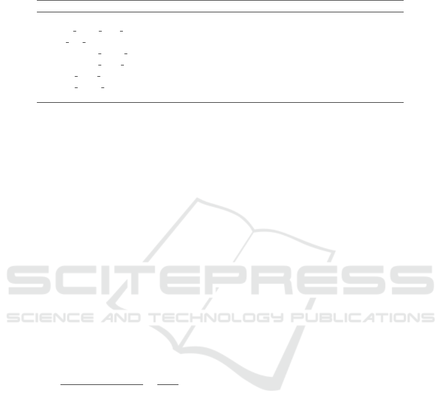
Table 2: Hyperparameter values adjusted in Mask R-CNN training for quasi-particles. The TRAIN columns symbolize each

of the training.

HYPERPARAMETERS TRAIN 1 TRAIN 2 TRAIN 3 TRAIN 4

BACKBONE ResNet101 ResNet50 ResNet101 ResNet50

TRAIN ROIS PER IMAGE 500 500 500 500

MAX GT INSTANCES 300 300 300 300

DETECTION MAX INSTANCES 500 500 500 500

DETECTION MIN CONFIDENCE 0.7 0.7 0.7 0.7

IMAGE MIN DIM 800 800 800 800

IMAGE MAX DIM 1024 1024 1024 1024

EPOCHS 50 50 100 100

4.4 Evaluation Criteria

For the graphical visualization of model losses, we

use Tensorboard. The loss of Mask R-CNN is calcu-

lated according to Equation 1. In deﬁned multitasking

loss, Lcls is rank loss, Lbox is bounding box loss, and

Lmask is mask loss (He et al., 2017).

L = L

cls

+ L

box

+ L

mask

(1)

To assess the precision of the model, we used the

mAP metric, which is a metric often used in object

recognition tasks. During detection, we seek to pre-

dict bounding boxes that overlap the labeled funda-

mental truth.

We can predict how good this overlap is by divid-

ing the area of the overlap by the total area of both

bounding boxes, giving the IoU (Intersection over

Union) metric as shown in Equation 2. It is common

for datasets to predeﬁne an IoU threshold of 0.5 when

sorting whether the prediction is a true positive or a

false positive.

IoU =

Area o f Intersection

Area o f Union

A ∩ B

A ∪ B

(2)

In image detection, precision refers to the per-

centage of bounding boxes predicted correctly (IoU

> 0.5) about all bounding boxes predicted in the im-

age, while recall is the percentage of bounding boxes

predicted correctly (IoU > 0.5) of all objects in the

image.

The IoU metric is the threshold for a correct pre-

diction. Thus, we can plot a precision versus recall

curve by the 0.5 IoU limit. This representation pro-

vides a curve with zigzag behavior for detection mod-

els, although it may vary for other models.

We then maximized the recall value for each pre-

cision value to smooth the curve’s behavior. The area

below the curve gives the average precision value, that

is, the average precision, metric AP (Average Preci-

sion). The average of the AP metric across all images

in a dataset gives the mAP metric (Mean Average Pre-

cision). We use the mAP metric to evaluate the model

against the labeled validation dataset.

5 RESULTS

In this section, we present the results obtained with

the implementation of the segmentation model. Pre-

liminary results indicated that instance segmentation

is an adequate approach for quasi-particle individual-

ization and separation by size classes. Next, we de-

scribe the results of the segmentation masks, classes,

evaluation metrics, and histograms generated by the

Tensorboard.

5.1 Segmentation

We performed the training with the adjusted hyper-

parameters, shown in Section 3.2. The results showed

that the segmentation masks converged with the edges

of the quasi-particles and with the segmented in-

stances separately, highlighting the class and the con-

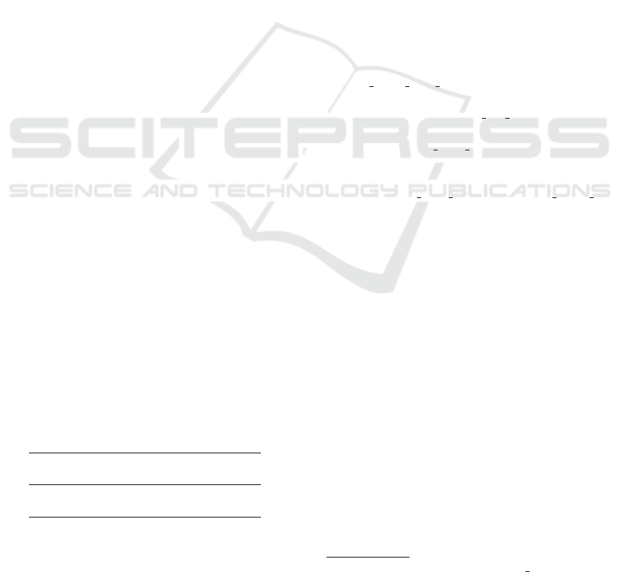
ﬁdence of the class, as shown in Figure 1. The edges

were well deﬁned, especially for the larger particles.

The models were also accurate in avoiding the de-

tection and segmentation of occluded and overlapping

particles, a factor that could lead to errors incorrectly

identifying the class.

5.2 Tensorboard

We visualize the values of training and validation

losses with the help of the Tensorboard tool. In the

graphs, the x-axis represents the number of training

epochs and the y-axis represents the loss values. The

loss values obtained by Mask RCNN are shown in Ta-

ble 3.

The training loss values were between 0.5663 and

0.7702, in which the smallest loss was recorded in

training 3, with the ResNet101 backbone and 100

Mask R-CNN Applied to Quasi-particle Segmentation from the Hybrid Pelletized Sinter (HPS) Process

465

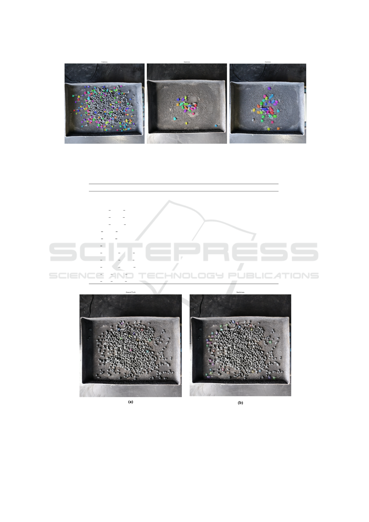
Figure 1: The prediction correctly demonstrates the masks as instances of the same class, the bounding box, and the predicted

conﬁdence results. The image was taken from training 3.

Table 3: Loss values obtained in the 4 training sessions performed. The highlighted values represent the lowest value for the

selected loss.

LOSSES TRAIN 1 TRAIN 2 TRAIN 3 TRAIN 4

50 epoch 50 epoch 100 epoch 100 epoch

loss 0.7702 0.7541 0.5663 0.5728

mrcnn bbox loss 0.06478 0.06426 0.031 0.03347

mrcnn class loss 0.1252 0.1221 0.077 0.0768

mrcnn mask loss 0.1567 0.1616 0.1215 0.1267

rpn bbox loss 0.3335 0.3062 0.2627 0.259

rpn class loss 0.08497 0.08507 0.07416 0.0768

val loss 0.8825 0.8783 0.8222 0.7977

val mrcnn bbox loss 0.1002 0.1001 0.0879 0.08419

val mrcnn class loss 0.1121 0.1259 0.1646 0.1446

val mrcnn mask loss 0.1657 0.1649 0.1684 0.1641

val rpn bbox loss 0.3875 0.3715 0.2952 0.3012

val rpn class loss 0.1168 0.1159 0.1061 0.1035

Figure 2: Example of an image containing particles of class 4-6’ from training 1. In a) the highlighted particles represent the

particles labeled and calculated as ground truth, and in b) the highlighted particles represent the particles found by the model

in predictions.

VISAPP 2022 - 17th International Conference on Computer Vision Theory and Applications

466

Figure 3: An example image of particles of class ‘8-9’ from training 4. In a) the highlighted particles as particles labeled and

calculated as ground truth, and in b) the highlighted particles represent the particles found by the model in the prediction.

training epochs. Losses for detection by bounding

boxes, generation of masks, and classiﬁcation were

quite positive, with the greatest loss for bounding

boxes in the RPN reﬁnement step. The graphics on

the tensorboard were smooth for losses.

The graphs generated on the Tensorboard for the

loss values for the validation showed ﬂuctuations,

mainly in the prediction of the classes in the val-

idation. This behavior can be associated with the

small number of labeling per image and the learning

rate. Thus, the suggestions for improving this valida-

tion ﬂuctuation behavior are annotation of a greater

amount of images and objects per image and a de-

crease in the learning rate during training.

The overall validation loss values were between

0.7977 and 0.8825. Training 2 recorded the least

loss, with the ResNet101 backbone and 100 training

epochs.

Table 4 shows the time of each training accord-

ing to the number of epochs. The number of epochs

was decisive in the execution time of the training time,

while the number of layers initialized by the Mask R-

CNN backbone had no signiﬁcant impact. Compared

with the general loss values “loss” for training and

“val loss” for validation, there was a decrease in loss

with the increase in the number of times trained, with

a single counterpart of the increase in model execu-

tion time.

We obtained the general loss values for training

(loss) and validation (val loss) in the graphs generated

by the Tensorboard, in Figures 4 and 5. The training

graphs demonstrate a smooth descent to model con-

vergence. We did not observe the same behavior in

the validation step loss graphs, with constant ﬂuctua-

tions and increase after a certain number of epochs.

Table 4: Training execution time according to the backbone

and number of epochs selected.

training backbone epochs time to execution

TRAIN 1 ResNet101 50 1h 33m 29s

TRAIN 2 ResNet50 50 1h 33m 7s

TRAIN 3 ResNet101 100 3h 9m 13s

TRAIN 4 ResNet50 100 3h 9m 29s

5.3 Model Performance

To assess the performance of the model, we use the

mAP metric with an IoU of 0.5. We obtained the ones

for the 46 images in the validation set. The values

obtained in each training are in Table 5.

Table 5: mAP metric values obtained for each training.

training backbone epochs mAP

TRAIN 1 ResNet101 50 0.2334

TRAIN 2 ResNet50 50 0.2585

TRAIN 3 ResNet101 100 0.2333

TRAIN 4 ResNet50 100 0.2511

The mAP metric values were close for all training,

and training 2 with ResNet50 and 50 epochs had the

highest value. However, there was a discrepancy that

impacted the mAP values. Images containing smaller

particles, from the ﬁrst three size classes, contained

much more particles (objects per image) than images

with larger particles, as the representations followed

the sampling: for each sample containing 1Kg of ma-

terial, proportionally, there are fewer particles of par-

ticle size greater than 6mm.

Mask R-CNN Applied to Quasi-particle Segmentation from the Hybrid Pelletized Sinter (HPS) Process

467

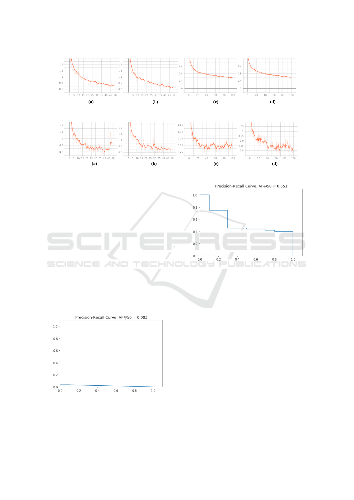
Figure 4: The graphs represent the overall training loss: a) training 1; b) training 2; c) training 3, and; d) training 4.

Figure 5: The graphs represent the general loss of validation: a) training 1; b) training 2; c) training 3, and; d) training 4.

Thus, with only ten annotations on each image in

the validation set, even though the model predicted

many more particles than annotated, the mAP of these

images were very small values. An example can be

seen in Figure 2, where the prediction predicted many

more particles than those labeled as ground truth.

The image in Figure 2 reached an AP of only

0.003 for an IoU of 0.5, showing the practical result

of this discrepancy as shown in Figure 6.

For the cases of images containing larger parti-

cles, such as those of the ‘>9’ class, the AP values

per image were higher, reaching 90% for some im-

ages. This is because almost all particles in the image

were labeled, so the chance of being contained in the

prediction was also greater (Figure 3).

Figure 7 shows the result of the AP metric in Fig-

ure 3 on the precision-recall curve, with AP value

equal to 0.551, that is, AP50= 55.1%, revealing the

discrepancy with Figure 6.

Figure 6: The precision-recall curve for the image in Figure

Thus, the Mask R-CNN architecture was able to

detect and segment the quasi-particles, as well as cor-

Figure 7: The precision-recall curve for the image in Figure

rectly classify the labeled classes, providing coherent

results.

6 CONCLUSION

In this work, we propose to obtain the quasi-particle

size in an imaging method based on the implementa-

tion of the Mask R-CNN algorithm for the detection

and segmentation of the quasi-particles according to

the desired class. To do so, we label the dataset by

classes according to the speciﬁed particle size range.

We performed four training sessions with hyper-

parameters adjusted and customized for the problem.

The model evaluation demonstrated good detection

and segmentation, correctly predicted classes, and

well-deﬁned quasi-particle edges. The model also had

good results by avoiding the segmentation of overlap-

ping and occluded particles, a factor that could lead

to the wrong prediction of the class.

VISAPP 2022 - 17th International Conference on Computer Vision Theory and Applications

468

The mAP metric used in evaluating the Mask R-

CNN model customized for this problem had results

between 0.2333 and 0.2585 for an IoU of 0.5. In the

individual evaluation of the AP metric of each image,

we veriﬁed that the AP values were lower for images

that contained many particles present in the sample

and higher AP values for images that contained few

particles present.

This factor may be associated with a small number

of labels in the validation set (only 10 per image), in-

creasing the probability for images with few particles

that the predicted value was associated with labeled

ground truth. For better AP results for these classes,

we suggest in future work that a greater proportion of

particles be labeled in the validation set and that the

training and validation sets have particles from differ-

ent classes labeled in the same image.

We emphasize that our implementation has the

challenge of working with images derived from an

industrial environment. These images are complex,

as they present homogeneity in color, texture, com-

plex background, overlapping, and occlusion. Fur-

thermore, we did not ﬁnd any database available for

the implementation, and we designed our database.

From the results obtained in this step, it was pos-

sible to raise new hypotheses of approaches to im-

prove the algorithm to obtain the particle size distri-

bution of the quasi-particles present in a sample in fu-

ture work. The development of applied solutions with

deep learning can bring signiﬁcant beneﬁts, both in

the improvement of processes and in the insertion of

steelmaking processes in Industry 4.0.

REFERENCES

Bello, R.-W., Mohamed, A. S. A., and Talib, A. Z. (2021).

Contour extraction of individual cattle from an im-

age using enhanced mask r-cnn instance segmentation

method. IEEE Access, 9:56984–57000.

Chen, D., Guo, D., Liu, S., and Liu, F. (2020). Microstruc-

ture instance segmentation from aluminum alloy met-

allographic image using different loss functions. Sym-

metry, 12(4):639.

Cohn, R., Anderson, I., Prost, T., Tiarks, J., White, E., and

Holm, E. (2021). Instance segmentation for direct

measurements of satellites in metal powders and au-

tomated microstructural characterization from image

data. JOM, pages 1–14.

De Cesaro J

unior, T. et al. (2020). Insectcv: um sistema

para detecc¸

ao de insetos em imagens digitais.

Girshick, R. (2015). Fast r-cnn. In Proceedings of the IEEE

international conference on computer vision, pages

1440–1448.

He, K., Gkioxari, G., Doll

ar, P., and Girshick, R. (2017).

Mask r-cnn. In Proceedings of the IEEE international

conference on computer vision, pages 2961–2969.

He, K., Zhang, X., Ren, S., and Sun, J. (2016). Deep resid-

ual learning for image recognition. In Proceedings of

the IEEE conference on computer vision and pattern

recognition, pages 770–778.

Johnson, J. W. (2018). Adapting mask-rcnn for au-

tomatic nucleus segmentation. arXiv preprint

arXiv:1805.00500.

LeCun, Y., Bengio, Y., and Hinton, G. (2015). Deep learn-

ing. nature, 521(7553):436–444.

Long, J., Shelhamer, E., and Darrell, T. (2015). Fully con-

volutional networks for semantic segmentation. In

Proceedings of the IEEE conference on computer vi-

sion and pattern recognition, pages 3431–3440.

Ren, S., He, K., Girshick, R., and Sun, J. (2015). Faster

r-cnn: Towards real-time object detection with region

proposal networks. Advances in neural information

processing systems, 28:91–99.

Soloy, A., Turki, I., Fournier, M., Costa, S., Peuziat, B.,

and Lecoq, N. (2020). A deep learning-based method

for quantifying and mapping the grain size on pebble

beaches. Remote Sensing, 12(21):3659.

Tu, S., Yuan, W., Liang, Y., Wang, F., and Wan, H.

(2021). Automatic detection and segmentation for

group-housed pigs based on pigms r-cnn. Sensors,

21(9):3251.

Vuola, A. O., Akram, S. U., and Kannala, J. (2019). Mask-

rcnn and u-net ensembled for nuclei segmentation. In

2019 IEEE 16th International Symposium on Biomed-

ical Imaging (ISBI 2019), pages 208–212. IEEE.

Wu, Q., Feng, D., Cao, C., Zeng, X., Feng, Z., Wu, J.,

and Huang, Z. (2021). Improved mask r-cnn for air-

craft detection in remote sensing images. Sensors,

21(8):2618.

Xi, D., Qin, Y., and Wang, Y. (2020). Vision measurement

of gear pitting under different scenes by deep mask

r-cnn. Sensors, 20(15):4298.

Xie, S., Girshick, R., Doll

ar, P., Tu, Z., and He, K. (2017).

Aggregated residual transformations for deep neural

networks. In Proceedings of the IEEE conference on

computer vision and pattern recognition, pages 1492–

1500.

Xu, B., Wang, W., Falzon, G., Kwan, P., Guo, L., Sun, Z.,

and Li, C. (2020). Livestock classiﬁcation and count-

ing in quadcopter aerial images using mask r-cnn. In-

ternational Journal of Remote Sensing, 41(21):8121–

8142.

Zhang, Q., Liu, Y., Gong, C., Chen, Y., and Yu, H. (2020).

Applications of deep learning for dense scenes analy-

sis in agriculture: A review. Sensors, 20(5):1520.

Zhang, R., Cheng, C., Zhao, X., and Li, X. (2019).

Multiscale mask r-cnn–based lung tumor detec-

tion using pet imaging. Molecular imaging,

18:1536012119863531.

Zhao, K., Kang, J., Jung, J., and Sohn, G. (2018). Building

extraction from satellite images using mask r-cnn with

building boundary regularization. In Proceedings of

the IEEE Conference on Computer Vision and Pattern

Recognition Workshops, pages 247–251.

Mask R-CNN Applied to Quasi-particle Segmentation from the Hybrid Pelletized Sinter (HPS) Process

469