Lossy Compressor Preserving Variant Calling through Extended BWT

Veronica Guerrini

1 a

, Felipe A. Louza

2 b

and Giovanna Rosone

1 c

Department of Computer Science, University of Pisa, Italy

Faculty of Electrical Engineering, Federal University of Uberl

andia, Brazil

Keywords:

eBWT, LCP, Positional Clustering, FASTQ, Smoothing, Noise Reduction, Compression.

Abstract:

A standard format used for storing the output of high-throughput sequencing experiments is the FASTQ for-

mat. It comprises three main components: (i) headers, (ii) bases (nucleotide sequences), and (iii) quality

scores. FASTQ ﬁles are widely used for variant calling, where sequencing data are mapped into a reference

genome to discover variants that may be used for further analysis. There are many specialized compressors

that exploit redundancy in FASTQ data with the focus only on either the bases or the quality scores compo-

nents. In this paper we consider the novel problem of lossy compressing, in a reference-free way, FASTQ data

by modifying both components at the same time, while preserving the important information of the original

FASTQ. We introduce a general strategy, based on the Extended Burrows-Wheeler Transform (EBWT) and

positional clustering, and we present implementations in both internal memory and external memory. Exper-

imental results show that the lossy compression performed by our tool is able to achieve good compression

while preserving information relating to variant calling more than the competitors.

Availability: the software is freely available at https://github.com/veronicaguerrini/BFQzip.

1 INTRODUCTION

The recent improvements in high-throughput se-

quencing technologies have led a reduced cost of

DNA sequencing and unprecedented amounts of ge-

nomic datasets, which has motivated the development

of new strategies and tools for compressing these data

that achieve better results than general-purpose com-

pression tools – see (Numanagi

c et al., 2016; Hernaez

et al., 2019) for good reviews.

FASTQ is the standard text-based format used to

store raw sequencing data, each DNA fragment (read)

is stored in a record composed by three main com-

ponents: (i) read identiﬁer with information related

to the sequencing process (header), (ii) nucleotide

sequence (bases), and (iii) quality sequence, with a

per-base estimation of sequencing conﬁdence (qual-

ity scores). The last two components are divided by

a “separator” line, which is generally discarded by

compressors as it contains only a “+” symbol option-

ally followed by the same header.

The majority of compressors for FASTQ ﬁles

commonly split the data into those three main com-

https://orcid.org/0000-0001-8888-9243

https://orcid.org/0000-0003-2931-1470

https://orcid.org/0000-0001-5075-1214

ponents (or streams), and compress them separately,

which allows much better compression rates.

The headers can be efﬁciently compressed taking

advantage of their structure and high redundancy. A

common strategy used by FASTQ compressors, like

SPRING (Chandak et al., 2018) and FaStore (Roguski

et al., 2018), is to tokenize each header: the sepa-

rators are non-alphanumerical symbols (Bonﬁeld and

Mahoney, 2013).

The bases and quality scores are commonly pro-

cessed separately, although their information are cor-

related, and current specialized compressors only fo-

cus on one of these two components.

Most of FASTQ compressors limit their focus on

the bases, compressing the quality scores indepen-

dently with a third tool or standard straightforward

techniques. The approaches that focus on compres-

sion the bases component are lossless, i.e., they do

not modify the bases, but they ﬁnd a good strategy to

represent the data by exploiting the redundancy of the

DNA sequences. An interesting strategy is to reorder

the sequences in the FASTQ ﬁle to gather reads orig-

inating from close regions of the genome (Cox et al.,

2012; Roguski et al., 2018; Hach et al., 2012; Chan-

dak et al., 2018).

Guerrini, V., Louza, F. and Rosone, G.

Lossy Compressor Preserving Variant Calling through Extended BWT.

DOI: 10.5220/0010834100003123

In Proceedings of the 15th International Joint Conference on Biomedical Engineering Systems and Technologies (BIOSTEC 2022) - Volume 3: BIOINFORMATICS, pages 38-48

ISBN: 978-989-758-552-4; ISSN: 2184-4305

On the other hand, approaches that focus on com-

pression the quality score component are generally

lossy, i.e., they modify the data by smoothing the

quality scores whenever possible. These approaches

can be reference-based when they use external infor-

mation (besides the FASTQ itself), such as a reference

corpus of k-mers, e.g. QUARTZ (Yu et al., 2015),

GeneCodeq (Greenﬁeld et al., 2016) and YALFF

(Shibuya and Comin, 2019). While, reference-free

strategies evaluate only the quality scores informa-

tion, such as the quantization of quality values using

QVZ (Malysa et al., 2015), Illumina 8-level binning

and binary thresholding, or evaluate the related bio-

logical information in the bases component (strate-

gies known as read-based) – e.g. BEETL (Janin et al.,

2014) and LEON (Benoit et al., 2015).

Our Contribution. In this work, we focus on a

novel approach for the lossy compression of both the

bases and the quality scores components taking into

account both information at the same time. In fact,

the two components are highly correlated being the

second one a conﬁdence estimation of each base call

contained in the ﬁrst one. To the best of our knowl-

edge, none of the existing FASTQ compressor tools

evaluates and modiﬁes both components at the same

time.

Note that we are not interested in compressing the

headers component, for which one can use any state-

of-the-art strategies or ignore them. Indeed, headers

can be artiﬁcially structured in ﬁelds to store informa-

tion only related to the sequencing process.

We focus on lossy reference-free and read-based

FASTQ compression that makes clever modiﬁcations

on the data, by reducing noise in the bases compo-

nent that could be introduced by the sequencer, and

by smoothing irrelevant values on the quality scores

component, according to the correlated information

in the bases, that would guarantee to preserve variant

calling.

Hence, we propose a novel read-based, reference-

and assembly-free compression approach for FASTQ

ﬁles, BFQZIP, which combines both DNA bases and

quality information for obtaining a lossy compressor.

Similarly to BEETL (Janin et al., 2014), our ap-

proach is based on the Extended Burrows-Wheeler

Transform (EBWT) (Burrows and Wheeler, 1994;

Mantaci et al., 2007) and its combinatorial properties,

and it applies the idea that each base in a read can with

high probability be predicted by the context of bases

that are next to it. We also exploit the fact that such

predicted bases add little information, and its quality

score can be discarded or heavily compressed without

distortion effects on downstream analysis.

In our strategy, the length of contexts is variable-

order (i.e. not ﬁxed a priori, unlike BEETL), and can

be as large as the full read length for high-enough cov-

erages and small-enough error rates.

We exploit the positional clustering framework in-

troduced in (Prezza et al., 2019) to detect “relevant”

blocks in the EBWT. These blocks allow us not only

to smooth the quality scores, but also to apply a noise

reduction on the corresponding bases, replacing those

that are believed to be noise, while keeping variant

calling performance comparable to that with the orig-

inal data and with compression rates comparable to

other tools.

2 PRELIMINARIES

Let S be a string (also called sequence or reads due to

our target application) of length n on the alphabet Σ.

We denote the i-th symbol of S by S[i]. A substring

of any S ∈ S is denoted as S[i, j] = S[i]···S[ j], with

S[1, j] being called a preﬁx and S[i,n + 1] a sufﬁx of S.

Let S = {S

,. . . , S

} be a collection of m

strings. We assume that each string S

∈ S has length

and is followed by a special end-marker symbol

+1] = $

, which is lexicographically smaller than

any other symbol in S , and does not appear in S else-

where.

The Burrows-Wheeler Transform (BWT) (Bur-

rows and Wheeler, 1994) of a text T (and the EBWT

of a set of strings S (Mantaci et al., 2007; Bauer

et al., 2013)) is a suitable permutation of the sym-

bols of T (and S ) whose output shows a local simi-

larity, i.e. symbols preceding similar contexts tend to

occur in clusters. Both transformations have been in-

tensively studied from a theoretical and combinatorial

viewpoint and have important and successful applica-

tions in several areas, e.g. (Mantaci et al., 2008; Li

and Durbin, 2010; Kimura and Koike, 2015; Shibuya

and Comin, 2019; Gagie et al., 2020; Guerrini et al.,

2020).

We assume that N =

∑

i=1

+1) denotes the sum

of the lengths of all strings in S . The output of

the EBWT is a string ebwt(S ) of length N such that

ebwt(S )[i] = x, with 1 ≤ i ≤ N, if x circularly pre-

cedes the i-th sufﬁx (context) S

[k, n

+ 1] (for some

1 ≤ j ≤ m and 1 ≤ k ≤ n

+1), according to the lexi-

cographic sorting of the contexts of all strings in S . In

this case, we say that the context S

[k, n

+ 1] is asso-

ciated with the position i in ebwt(S ). See Table 1 for

an example.

In practice, computing the EBWT via sufﬁx sort-

ing (Bauer et al., 2013; Bonomo et al., 2014) may be

done considering the same end-markers for all strings.

Lossy Compressor Preserving Variant Calling through Extended BWT

Table 1: Extended Burrows-Wheeler Transform (EBWT), LCP array, and auxiliary data structures used for detecting posi-

tional clusters for the set S = {GGCGTACCA$

,GGGGCGTAT $

,ACGANTACGAC$

} and k

= 2.

i B

min

thr

lcp ebwt Sorted Sufﬁxes i B

min

thr

lcp ebwt Sorted Sufﬁxes

1 0 0 0 A $

17 0 1 4 G C G T A T $

2 0 0 0 T $

18 1 0 0 C G A C$

3 0 0 0 C $

19 0 1 2 C G A N T A C G A C $

4 0 0 0 C A$

20 1 0 1 G G C G T A C C A$

5 0 0 1 G A C$

21 0 1 5 G G C G T A T $

6 0 1 2 T A C C A$

22 1 0 1 $ GG C G T A C C A$

7 0 1 2 T A C G A C $

23 0 1 6 G G G C G T A T $

8 0 1 4 $ A C G A N T A C GAC $

24 1 1 2 G G G G C G T A T $

9 1 0 1 G A N T A C GA C $

25 0 1 3 $ GGGG C G T A T $

10 0 0 1 T A T $

26 1 0 1 C G T A C C A$

11 1 0 0 A C$

27 0 1 3 C G T A T $

12 0 0 1 C C A$

28 1 0 0 A N T A C G A C $

13 0 0 1 A C C A$

29 0 0 0 A T$

14 0 0 1 A C G A C $

30 0 0 1 G T A C C A$

15 0 1 3 A C G A N T A C G AC$

31 0 1 3 N T A C G A C $

16 1 1 2 G C G T A C C A$

32 0 1 2 G T A T$

That is, we assume that $

< $

, if i < j, and use a

unique symbol $ as the end-marker for all strings.

The longest common preﬁx (LCP) array (Manber

and Myers, 1990) of S is the array lcp(S ) of length

N +1, such that for 2 ≤ i ≤ N, lcp(S )[i] is the length of

the longest common preﬁx between the contexts asso-

ciated with the positions i and i − 1 in ebwt(S ), while

lcp(S )[1] = lcp(S )[N + 1] = 0. The LCP-intervals

(Abouelhoda et al., 2004) are maximal intervals [i, j]

that satisfy lcp(S )[r] ≥ k for i < r ≤ j and whose as-

sociated contexts share at least the ﬁrst k symbols.

An important property of the BWT and EBWT,

is the so-called LF mapping (Ferragina and Manzini,

2000), which states that the i-th occurrence of sym-

bol x on the BWT string and the ﬁrst symbol of the

i-th lexicographically-smallest sufﬁx that starts with

x correspond to the same position in the input string

(or string collection). We will use the LF mapping

to perform backward searches when creating a new

(modiﬁed) FASTQ ﬁle. The backward search allows

to ﬁnd the range of sufﬁxes preﬁxed by a given string

– see (Ferragina and Manzini, 2000; Adjeroh et al.,

2008) for more details.

3 METHOD

We structure our reference-free FASTQ compression

method in four main steps: (a) data structures build-

ing, (b) positional cluster detecting, (c) noise reduc-

tion and quality score smoothing, and (d) FASTQ re-

construction.

(a) Data Structures Building. This phase consists

in computing the EBWT and the LCP array for the

collection of sequences S stored in the bases compo-

nent of the input FASTQ ﬁle. We also compute qs(S ),

as the concatenation of the quality scores associated

with each symbol in ebwt(S ), i.e., the string qs con-

tains a permutation of the quality score symbols that

follows the symbol permutation in ebwt(S ). Note that

the lcp(S ) is only used in the next step, so we can ei-

ther explicitly compute it in this phase or implicitly

deduce it by ebwt(S ) during the next step.

(B) Positional Cluster Detecting. A crucial prop-

erty of the EBWT is that symbols preceding sufﬁxes

that begin with the same substring (context) w will

result in a contiguous substring of ebwt, and thus of

qs. Such a substring of the ebwt is generally called

cluster. In literature, such clusters depending on the

length k of the context w are associated with LCP-

intervals (Abouelhoda et al., 2004).

The aim of the positional clustering frame-

work (Prezza et al., 2019; Prezza et al., 2020) is to

overcome the limitation of strategies based on LCP-

intervals, which depend on the choice of k. Intuitively,

meaningful clusters in the EBWT lie between local

minima in the LCP array, and symbols of the same

positional cluster usually cover the same genome lo-

cation (Prezza et al., 2019). This recent strategy au-

tomatically detects, in a data-driven way, the length k

of the common preﬁx shared by the sufﬁxes of a clus-

ter in the EBWT. Moreover, so as to exclude clusters

corresponding to short random contexts, we set a min-

imum length for the context w, denoted by k

Analogously to (Prezza et al., 2020), we deﬁne

positional clusters by using two binary vectors: B

thr

and B

min

, where B

thr

[i] = 1 if and only if lcp[i] ≥ k

and B

min

= 1 if and only if lcp[i] is a local mini-

BIOINFORMATICS 2022 - 13th International Conference on Bioinformatics Models, Methods and Algorithms

mum i.e., it holds lcp[i − 1] > lcp[i] ≤ lcp[i +1], for all

1 < i ≤ N, which depends on data only. A EBWT po-

sitional cluster is a maximal substring ebwt[i, j] such

that B

thr

[r] = 1, for all i < r ≤ j, and B

min

[r] = 0, for

all i < r ≤ j. See, for instance, Table 1.

(C.1) Noise Reduction. Given the base symbols ap-

pearing in any positional cluster of ebwt(S ), we call

as frequent symbol any symbol whose occurrence in

the cluster is greater than a threshold percentage. The

idea that lies behind changing bases is to reduce the

number of symbols in a cluster that are different from

the most frequent symbols, while preserving the vari-

ant calls. So, we take into account only clusters that

have no more than two frequent symbols (for exam-

ple, we set the threshold percentage to 40%).

The symbols in an EBWT positional cluster usu-

ally correspond to the same genome location (Prezza

et al., 2019). Thus, given an EBWT positional cluster

α = ebwt[i, j], we say a symbol b is a noisy base if

it is different from the most frequent symbols and all

occurrences of b in α are associated with low qual-

ity values in qs[i, j] (i.e. there are no occurrences of

b with a high quality score in α). Intuitively, a noisy

base is more likely noise introduced during the se-

quencing process.

Then, for each analyzed cluster α, we replace

noisy bases in α with a predicted base c as follows.

We distinguish two cases. If the cluster α contains a

unique most frequent symbol c, then we replace the

noisy base b with c. Otherwise, if we have two dif-

ferent frequent symbols, for each occurrence of them

and for the noisy base b, we compute the preceding

context of length ` in their corresponding reads (i.e.

left context of each considered base), by means of the

backward search applied to ebwt(S) (for example, we

set ` = 1 in our experiments). If the left context pre-

ceding b coincides with the contexts preceding all the

occurrences of d (one of the two most frequent sym-

bols), then we replace the base b with d. We spec-

ify that no base changes are performed if the frequent

symbols are preceded by the same contexts.

(C.2) Quality Score Smoothing. During step (c.1),

we also modify quality scores by smoothing the sym-

bols of qs that are associated with base symbols in

clusters of ebwt.

In any cluster α, the value Q used for replacements

can be computed with different strategies: (i) Q is a

default value, or (ii) Q is the quality score associated

with the mean probability error in α, or (iii) Q is the

maximum quality score in α, or (iv) Q is the average

of the quality scores in α. According to this smooth-

ing process, apart from strategy (i), the value Q de-

pends on the cluster analyzed. In the experiments we

evaluated qs smoothing as follows. For each position

r within α = ebwt[i, j] we smooth the quality score

qs[r] with Q, either if ebwt[r] is one of the most fre-

quent symbols (regardless of its quality), or if qs[r] is

greater than Q.

An additional feature to compress further quality

scores is the possibility of reducing the number of the

alphabet symbols appearing in qs(S ). This smooth-

ing approach is quite popular and standard in litera-

ture (Chandak et al., 2018). Then, in addition to one

of the strategies described above, we can apply the Il-

lumina 8-level binning reducing to 8 the number of

different symbols in qs.

(D) FASTQ Reconstruction and Compression.

Given the modiﬁed symbols in ebwt(S ) and in qs(S )

(according to the strategies described above), we use

the LF mapping on the original ebwt string to retrieve

the order of symbols and output a new (modiﬁed)

FASTQ ﬁle.

The headers component with the read titles can be

either omitted (inserting the symbol ‘@’ as header) or

kept as they are in the original FASTQ ﬁle.

At the end, the resulting FASTQ ﬁle is com-

pressed by using any state-of-the-art compressor.

4 EXPERIMENTS

Implementations. We present two implementa-

tions of our tool BFQZIP: in internal memory and

in external memory. Now we give a brief description

of them.

Given a FASTQ ﬁle containing a collection S ,

both implementations take as input the ﬁles contain-

ing ebwt(S ) and qs(S ). In the external memory, we

also need the array lcp(S ).

The construction of these data structures dur-

ing the ﬁrst step can be performed with any tools.

e.g. (Bauer et al., 2013; Bonizzoni et al., 2019; Egidi

et al., 2019; Louza et al., 2020; Boucher et al., 2021)

according to the resources available (which is a good

feature).

The two implementations largely differ in the de-

tection of positional clusters. Indeed, alike (Prezza

et al., 2020), the internal memory approach rep-

resents ebwt(S ) via the compressed sufﬁx tree de-

scribed in (Prezza and Rosone, 2021) (see also (Be-

lazzougui et al., 2020)), where it is shown that lcp(S )

can be induced from the EBWT using succinct work-

ing space for any alphabet size. Whereas, in exter-

nal memory, EBWT positional clusters are detected

Lossy Compressor Preserving Variant Calling through Extended BWT

Table 2: Paired-end datasets used in the experiments and their sizes in bytes. Each dataset is obtained from two ﬁles ( 1 and

2), whose number of reads and read length are given in columns 2 and 3. We distinguish the size of the original FASTQ (raw

data) from the size of the same FASTQ ﬁle with all headers removed (i.e., replaced by ’@’). In the last column we report the

size of the bases component, that is equal to the quality scores component size.

Dataset No. reads Length Raw (complete) FASTQ DNA/QS

ERR262997 1 - chr 20 13,796,697 101 3,420,752,544 2,869,712,976 1,407,263,094

ERR262997 2 - chr 20 13,796,697 101 3,420,752,544 2,869,712,976 1,407,263,094

ERR262997 1 - chr 14 18,596,541 101 4,611,888,574 3,868,080,528 1,896,847,182

ERR262997 2 - chr 14 18,596,541 101 4,611,888,574 3,868,080,528 1,896,847,182

ERR262997 1 - chr 1 49,658,795 101 12,211,743,094 10,329,029,360 5,065,197,090

ERR262997 2 - chr 1 49,658,795 101 12,211,743,094 10,329,029,360 5,065,197,090

by reading the lcp(S ) stored in a ﬁle in a sequential

way.

For the last two steps, the two implementations

are similar, except that the data are kept in internal or

external memory. In particular, during step (d), we

use the LF-mapping either in internal memory – via

the sufﬁx-tree navigation as in (Prezza et al., 2020)

– or in external memory – similarly to (Bauer et al.,

2013).

Datasets. The easiest approach to evaluate the va-

lidity of our method could be to simulate reads and

variants from a reference genome. However, it is not

trivial to simulate variant artifacts for this purpose (Li,

2014), so we focus only on real data.

In this study, thus, we use the real human dataset

ERR262997 corresponding to a 30x-coverage paired-

end Whole Genome Sequencing (WGS) data for the

CEPH 1463 family. Similarly to other studies (Ochoa

et al., 2016), for evaluation purposes we extracted the

chromosomes 20, 14 and 1 from ERR262997, obtain-

ing datasets of different sizes (see Table 2).

Compression. We describe experiments that show

that our strategy is able to compress FASTQ ﬁles in

lossy way modifying both the bases and quality scores

component, while keeping most of the information

contained in the original ﬁle.

To the best of our knowledge, none of the existing

FASTQ compressors evaluates and modiﬁes both the

bases and the quality scores components at the same

time. Therefore, no comparison with existing tools is

completely fair. We consider the tools BEETL

(Janin

et al., 2014) and LEON

(Benoit et al., 2015) that are

reference-free and read-based: they smooth the qual-

ity score component in a lossy way based on the bi-

ological information of the bases, without modifying

the bases themselves.

https://github.com/BEETL/BEETL/blob/

RELEASE 1 1 0/scripts/lcp/applyLcpCutoff.pl

http://gatb.inria.fr/software/leon/

We choose BEETL, because it is based on EBWT

and takes as input the same data structures we com-

pute during step (a). BEETL smooths to a con-

stant value the quality scores corresponding to each

run of the same symbol associated with the LCP-

interval [i, j]. The quality scores associated to each

run in ebwt[i, j] are smoothed if the length of the run is

greater than a minimum stretch length s. So, it needs

two parameters: the minimum stretch length s and the

cut threshold c for the LCP-interval, failing to sepa-

rate read sufﬁxes differing after c positions (this is,

indeed, a drawback of all c-mer-based strategies).

We choose LEON (Benoit et al., 2015) that, on

the contrary, needs to build a reference from the in-

put reads in the form of a bloom ﬁlter compressed

de Bruijn graph, and then maps each nucleotide se-

quence as a path in the graph. Thus, LEON can be

considered assembly-based, since it uses a de Bruijn

graph as a de novo reference. If a base is covered by

a sufﬁciently large number of k-mers (substrings of

length k) stored in the bloom ﬁlter, its quality is set to

a ﬁxed high value. Thus, LEON depends on a ﬁxed

parameter k for the graph, as well.

Regarding the output of each tool, BFQZIP pro-

duces a new FASTQ ﬁle with modiﬁed bases and

smoothed qualities, whereas BEETL only produces a

BWT-ordered smoothed qualities ﬁle, which is used

to replace the quality scores component in the modi-

ﬁed FASTQ ﬁle (with the original bases component).

LEON produces a proprietary format compressed ﬁle

that encodes the de Bruijn graph, thus, it was neces-

sary to uncompress the output ﬁle to obtain the mod-

iﬁed FASTQ. For a fairer comparison, these resulting

FASTQ ﬁles were compressed with the same tools.

In particular, we choose two well-known compressors

for this task: PPMd (Cleary and Witten, 1984; Moffat,

1990) and BSC

We run BFQZIP and BEETL with similar param-

eters: in BEETL, we set the replacement quality score

to ‘@’ (as set by LEON) and the minimum LCP cut

threshold to 30. For BFQZIP, we used options -T 30

to set the minimum context length k

= 30 and -Q

http://libbsc.com/

BIOINFORMATICS 2022 - 13th International Conference on Bioinformatics Models, Methods and Algorithms

Table 3: Compression ratio for (original and three smoothing tools) FASTQ ﬁles (with headers replaced by ’@’) and their

single components (qualities (QS) and bases (DNA)) obtained by both PPMd and BSC. The ratio is deﬁned as compressed

size/original size, where original ﬁle size is in Table 2. Since BEETL and LEON do not modify the bases component, their

ratio for the DNA component is the same as the original.

Tool

FASTQ QS DNA FASTQ QS DNA

ERR262997 1 chr 20 ERR262997 2 chr 20

PPMd

Original 0.2473 0.2999

0.2037

0.2547 0.3142

0.2046LEON 0.1152 0.0317 0.1234 0.0473

BEETL 0.1900 0.1833 0.2002 0.2033

BFQZIP 0.1941 0.1918 0.2035 0.2043 0.2119 0.2043

BSC

Original 0.2005 0.2902

0.1154

0.2095 0.3034

0.1207LEON 0.0677 0.0241 0.0780 0.0394

BEETL 0.1413 0.1724 0.1534 0.1915

BFQZIP 0.1453 0.1830 0.1152 0.1572 0.2024 0.1200

ERR262997 1 chr 14 ERR262997 2 chr 14

PPMd

Original 0.2482 0.2956

0.2100

0.2544 0.3076

0.2106LEON 0.1175 0.0301 0.1249 0.0444

BEETL 0.1916 0.1805 0.2010 0.1989

BFQZIP 0.1957 0.1889 0.2098 0.2050 0.2074 0.2103

BSC

Original 0.1992 0.2862

0.1174

0.2071 0.2972

0.1224LEON 0.0674 0.0226 0.0770 0.0367

BEETL 0.1406 0.1698 0.1518 0.1874

BFQZIP 0.1445 0.1786 0.1164 0.1555 0.1962 0.1210

ERR262997 1 chr 1 ERR262997 2 chr 1

PPMd

Original 0.2461 0.2969

0.2046

0.2529 0.3097

0.2054LEON 0.1148 0.0299 0.1224 0.0445

BEETL 0.1876 0.1777 0.1973 0.1966

BFQZIP 0.1918 0.1864 0.2044 0.2015 0.2054 0.2051

BSC

Original 0.1984 0.2874

0.1146

0.2068 0.2991

0.1197LEON 0.0661 0.0224 0.0758 0.0367

BEETL 0.1379 0.1669 0.1494 0.1850

BFQZIP 0.1419 0.1759 0.1136 0.1533 0.1941 0.1183

Table 4: Evaluation of called variants by means of rtg vcfeval: comparison between called variants from a modiﬁed

FASTQ and variants from the original FASTQ used as baseline.

ERR262997 chr 20 ERR262997 chr 14 ERR262997 chr 1

PREC SEN F PREC SEN F PREC SEN F

LEON 0.9593 0.9356 0.9473 0.9626 0.9381 0.9502 0.9589 0.9348 0.9467

BEETL 0.9584 0.9529 0.9556 0.9626 0.9553 0.9590 0.9596 0.9526 0.9561

BFQZIP 0.9613 0.9534 0.9574 0.9650 0.9555 0.9602 0.9628 0.9523 0.9575

@ to set the constant replacement value. LEON was

executed with default parameters for k-mer size and

minimal abundance threshold, as suggested by the au-

thors. The exact commands for the tools are:

• python3 BFQzip.py <input>.fastq -o

<output>.fastq -T 30 -Q @

• applyLcpCutoff.pl -b <input>.ebwt

-q <input>.ebwt.qs -l <input>.lcp -o

<output>.ebwt.qs -c 30 -r 64 -s 5

• leon -file <input>.fastq -c (for decom-

pression -d) -nb-cores 1

In Table 3, we report the compression ratios

achieved by PPMd and BSC given as input the

FASTQ modiﬁed by any of the three tools and the

original FASTQ ﬁle. Note that each of the two

FASTQ ﬁles comprising any paired-end dataset is

compressed separately.

Table 3 shows that all tools improve the compres-

sion of the data (compared with the original FASTQ).

In particular, LEON is better in terms of compres-

sion ratios than other tools. This improvement is

due to a greater ability to smooth the quality scores

component. Recall that LEON truncates all qual-

ity scores above a given threshold (qualities higher

than ‘@’ are replaced by ‘@’) and in these datasets

the total frequency of symbols greater than ‘@’ is

about 80− 90%. However, the results of BFQZIP and

BEETL were similar in almost all cases.

Validation. In lossy FASTQ compression, it is im-

portant to take into account the impact of the modiﬁed

data on downstream analysis, so we need to evaluate

the genotyping accuracy.

Lossy Compressor Preserving Variant Calling through Extended BWT

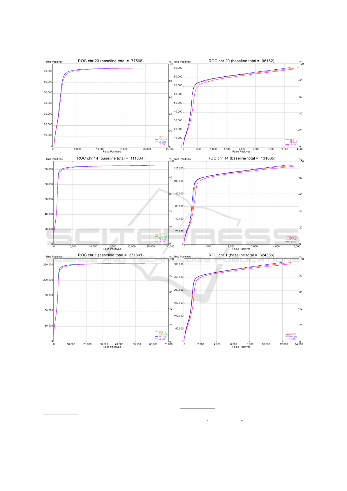
Figure 1: ROC Curves obtained by rtg rocplot: true positive as a function of the false positive respect both to the Ground

truth as baseline (left side) and to the original ﬁle as baseline (right side).

We compared the set of variants retrieved from

a baseline with the set retrieved from the modiﬁed

FASTQ. First, we considered as baseline the set of

“ground truth” variants for NA12878 provided by Il-

lumina

and then, we considered as baseline the set of

variants obtained from the original FASTQ ﬁles.

https://github.com/Illumina/PlatinumGenomes

The SNP calling pipeline is a bash script

(Li, 2013) to align sequences to the reference (in

our case, the latest build of the human reference

genome, GRCh38/hg38) and GATK-HaplotypeCaller

(DePristo and et al., 2011) to call SNPs. The output

https://github.com/veronicaguerrini/BFQzip/blob/

main/variant calling/pipeline SNPsCall.sh

BIOINFORMATICS 2022 - 13th International Conference on Bioinformatics Models, Methods and Algorithms

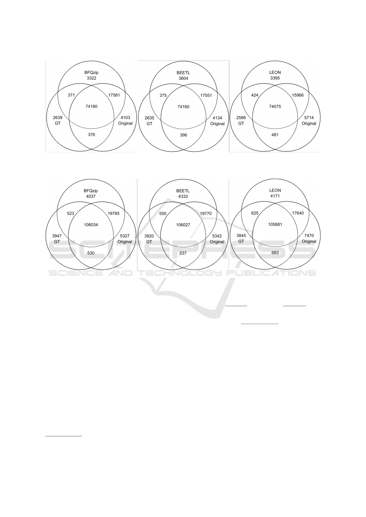
Figure 2: Venn diagrams for chr 20 variants: set comparison between the variants in the original FASTQ ﬁle (Original), those

in the ground truth (GT) and those called from the FASTQ modiﬁed by BFQzip (left), or modiﬁed by BEETL (middle), or

modiﬁed by LEON (right).

Figure 3: Venn diagrams for chr 14 variants: set comparison between the variants in the original FASTQ ﬁle (Original), those

in the ground truth (GT) and those called from the FASTQ modiﬁed by BFQzip (left), or modiﬁed by BEETL (middle), or

modiﬁed by LEON (right).

of the pipeline is a VCF ﬁle that contains the set

of called SNPs, which are then compared to those

contained in a baseline set by using RTG Tools

rtg vcfeval evaluates agreement between called

and baseline variants using the following performance

metrics.

True positive (T P) are those variants that match

in both baseline and query (the set of called variants);

false positives (FP) are those variants that have mis-

matching, that are in the called set of variants but

not in the baseline; false negatives (FN) are those

variants that are present in the baseline, but miss-

ing in the query. These values are employed to

compute precision (PREC) that measures the propor-

tion of called variants that are true, and sensitivity

(SEN), which measures the proportion of called vari-

ants included in the consensus set. A third metric is

the harmonic mean between sensitivity and precision

(known as F-measure):

https://www.realtimegenomics.com/products/rtg-tools

PREC =

T P

T P + FP

, SEN =

T P

T P + FN

F =

2 · SEN · PREC

SEN + PREC

The tool rtg vcfeval can also output a ROC ﬁle

based on the QUAL ﬁeld, which can be viewed by rtg

rocplot.

Table 4 reports the evaluation results of the vari-

ants retrieved from a modiﬁed FASTQ (produced by

any tool) compared to the set of variants from the

original (unsmoothed) FASTQ, which is used as base-

line. We observe that our method provides the highest

precision and F measure. This means that, with re-

spect to the original FASTQ, we have a higher num-

ber of common variants (TP) and the lowest number

of newly-introduced variants (FP), thus we preserve

information of the original FASTQ more than the oth-

ers (see also Figure 1, right side). This is a desirable

property useful in several applications.

Lossy Compressor Preserving Variant Calling through Extended BWT

In Figure 1 we provide the ROC curves associ-

ated with the variant comparison performed by rtg

vcfeval (reporting the number of TP as a function of

the FP), showing similar results.

Figure 1 (left side) shows that our tool preserves

those variants that are in the ground truth: using the

VCF ﬁle of the ground truth as baseline, all tools

show an accuracy similar to the original. In particular,

BFQZIP and BEETL curves in each graph overlap the

original one, while LEON’s curve is a bit lower.

Figure 1 (right side) also shows that our tool pre-

serves the original variants (TP) introducing only a

little number of new ones (FP) when the original

FASTQ variants are used as baseline (as also shown

by the percentages of sensitivity and precision in Ta-

ble 4) .

With the idea of showing the preservation of vari-

ants from the original ﬁle and the possibility of los-

ing variants due to the sequencer noise, we decided to

manually check the variants obtained for any tool by

intersecting the corresponding vcf ﬁle with that from

the FASTQ original and with the ground truth vcf.

Figures 2 and 3 show as our tool preserves the vari-

ants that are both in the original ﬁle and in the ground

truth (i.e. GT) more than the others.

This analysis appears to conﬁrm what we ob-

served with the ROC curves. BFQZIP reports the

smaller number of new variants introduced by the

tool, that are those variants neither in the original ﬁle

nor in the ground truth.

The majority of the variants present in both the

original FASTQ and the ground truth is preserved by

all tools. However, it appears that the heavy trunca-

tion of the quality scores carried out by LEON leads to

a loss of variants present in the original ﬁle (see, for

instance, the intersection between each tool and the

original, or the intersection between the ground truth

and the original). While BFQZIP (and in the simi-

lar way BEETL) preserves a high number of variants

that are present in the original ﬁle (see intersection

between each tool and the original).

We also made a detailed analysis of the modiﬁca-

tions performed by our method, comparing the modi-

ﬁed bases which correspond to parts aligned by BWA

with the relative bases in the reference (taking into ac-

count how BWA aligned the reads). We have noticed

that about 91-93% of the changed bases correspond to

the reference. The remaining part includes positions

we cannot evaluate, such as those in the reads skipped

by the aligner.

5 DISCUSSION AND

CONCLUSIONS

We propose the ﬁrst lossy reference-free and

assembly-free compression approach for FASTQ

ﬁles, which combines both DNA bases and quality in-

formation in the reads to smooth the quality scores

and to apply a noise reduction of the bases, while

keeping variant calling performance comparable to

that with original data. To the best of our knowledge,

there are no tools that have been designed for this pur-

pose, so we compared our results with two reference-

free and read-based tools that only smooth out the

quality scores component: BEETL (Janin et al., 2014)

and LEON (Benoit et al., 2015).

The resulting FASTQ ﬁle with the modiﬁed bases

and quality scores produced by our tool achieves bet-

ter compression than the original data. In particular,

by using our approach the bases component achieves

better compression than the original (therefore also

than competitors which do not make any changes to

this component), whereas the compression ratio of the

quality scores component is more competitive with

BEETL than LEON, which also truncates all quality

values greater than ‘@’. On the other hand, in terms

of variant calling, our tool keeps the same accuracy

as the original FASTQ data when the ground truth is

used as baseline, and preserves the variant calls of the

original FASTQ ﬁle better than BEETL and LEON.

From the viewpoint of the used resources, LEON

has shown to be the fastest tool, although this com-

parison is not completely fair because our tool mod-

iﬁes different components of the FASTQ ﬁle and the

outputs are different (not directly comparable). More-

over, the authors in (Benoit et al., 2015) state that for

WGS datasets, the relative contribution of the Bloom

ﬁlter is low for high coverage datasets, but prohibitive

for low coverage datasets (e.g. 10x). We intend to

improve our implementation also using, for instance,

parallelization, and test our tool for low coverage

datasets and longer reads.

Our implementations give as output the modiﬁed

FASTQ ﬁle, so we have used PPMd and BSC for

compression, but we could use any other compres-

sor for this task and we could also combine exist-

ing lossless compression schemes to further reduce

the size of the FASTQ ﬁle, for instance we could use

SPRING (Chandak et al., 2018), FQSquezeer (De-

orowicz, 2020), and others.

Moreover, our strategy could take advantage of

the reordering of the reads based on their similarity,

e.g. as in (Cox et al., 2012; Chandak et al., 2018;

Deorowicz, 2020). Another feature we did not ex-

ploit in our compression scheme is the paired-end in-

BIOINFORMATICS 2022 - 13th International Conference on Bioinformatics Models, Methods and Algorithms

formation coming from reads in pairs. (Indeed, we

compress the FASTQ ﬁles in a paired-end dataset in-

dependently, as they were single-end.) Both the above

aspects could be analyzed as future work.

We believe the results presented in this paper can

motivate the development of new FASTQ compres-

sors that modify the bases and quality scores com-

ponents taking into account both information at the

same time to achieve better compression while keep-

ing most of the relevant information in the FASTQ

data. As future work we intend to investigate the er-

ror correction problem that needs to take into account

much more information (e.g. reverse-complement, or

paired-end information).

ACKNOWLEDGEMENTS

The authors would like to thank N. Prezza for valu-

able comments and suggestions and for providing part

of the code library, and E. Niccoli for preliminary ex-

perimental investigations on positional clustering and

compression in his bachelor’s thesis under the super-

vision of GR and VG.

Work partially supported by the project MIUR-

SIR CMACBioSeq (“Combinatorial Methods for

Analysis and Compression of Biological Sequences”)

grant n. RBSI146R5L and by the University of Pisa

under the “PRA – Progetti di Ricerca di Ateneo” (In-

stitutional Research Grants) - Project no. PRA 2020-

2021 26 “Metodi Informatici Integrati per la Biomed-

ica”.

REFERENCES

Abouelhoda, M. I., Kurtz, S., and Ohlebusch, E. (2004). Re-

placing sufﬁx trees with enhanced sufﬁx arrays. Jour-

nal of Discrete Algorithms, 2(1):53 – 86.

Adjeroh, D., Bell, T., and Mukherjee, A. (2008). The

Burrows-Wheeler Transform: Data Compression,

Sufﬁx Arrays, and Pattern Matching. Springer.

Bauer, M., Cox, A., and Rosone, G. (2013). Lightweight

algorithms for constructing and inverting the BWT of

string collections. Theor. Comput. Sci., 483(0):134 –

148.

Belazzougui, D., Cunial, F., K

arkk

ainen, J., and M

akinen,

V. (2020). Linear-time string indexing and analysis in

small space. ACM Trans. Algorithms, 16(2).

Benoit, G., Lemaitre, C., Lavenier, D., Drezen, E., Dayris,

T., Uricaru, R., and Rizk, G. (2015). Reference-free

compression of high throughput sequencing data with

a probabilistic de bruijn graph. BMC Bioinformatics,

16.

Bonﬁeld, J. K. and Mahoney, M. V. (2013). Compression of

FASTQ and sam format sequencing data. PLOS ONE,

8(3).

Bonizzoni, P., Della Vedova, G., Pirola, Y., Previtali,

M., and Rizzi, R. (2019). Multithread Multistring

Burrows-Wheeler Transform and Longest Common

Preﬁx Array. Journal of computational biology,

26(9):948—961.

Bonomo, S., Mantaci, S., Restivo, A., Rosone, G., and

Sciortino, M. (2014). Sorting conjugates and sufﬁxes

of words in a multiset. International Journal of Foun-

dations of Computer Science, 25(08):1161–1175.

Boucher, C., Cenzato, D., Lipt

ak, Z., Rossi, M., and

Sciortino, M. (2021). Computing the original ebwt

faster, simpler, and with less memory. In SPIRE, pages

129–142. Springer International Publishing.

Burrows, M. and Wheeler, D. (1994). A Block Sorting data

Compression Algorithm. Technical report, DIGITAL

System Research Center.

Chandak, S., Tatwawadi, K., Ochoa, I., Hernaez, M.,

and Weissman, T. (2018). SPRING: a next-

generation compressor for FASTQ data. Bioinformat-

ics, 35(15):2674–2676.

Cleary, J. and Witten, I. (1984). Data compression using

adaptive coding and partial string matching. IEEE

Transactions on Communications, 32(4):396–402.

Cox, A., Bauer, M., Jakobi, T., and Rosone, G.

(2012). Large-scale compression of genomic se-

quence databases with the Burrows-Wheeler trans-

form. Bioinformatics, 28(11):1415–1419.

Deorowicz, S. (2020). Fqsqueezer: k-mer-based compres-

sion of sequencing data. Scientiﬁc reports, 10(1):1–9.

DePristo, M. A. and et al. (2011). A framework for variation

discovery and genotyping using next-generation DNA

sequencing data. Nature genetics, 43(5):491–498.

Egidi, L., Louza, F. A., Manzini, G., and Telles, G. P.

(2019). External memory BWT and LCP computation

for sequence collections with applications. Algorithms

for Molecular Biology, 14(1):6:1–6:15.

Ferragina, P. and Manzini, G. (2000). Opportunistic data

structures with applications. In FOCS, pages 390–

398. IEEE Computer Society.

Gagie, T., Navarro, G., and Prezza, N. (2020). Fully Func-

tional Sufﬁx Trees and Optimal Text Searching in

BWT-Runs Bounded Space. J. ACM, 67(1):2:1–2:54.

Greenﬁeld, D. L., Stegle, O., and Rrustemi, A. (2016).

GeneCodeq: quality score compression and improved

genotyping using a Bayesian framework. Bioinfor-

matics, 32(20):3124–3132.

Guerrini, V., Louza, F., and Rosone, G. (2020). Metage-

nomic analysis through the extended Burrows-

Wheeler transform. BMC Bioinformatics, 21.

Hach, F., Numanagi

c, I., Alkan, C., and Sahinalp, S. C.

(2012). SCALCE: boosting sequence compression al-

gorithms using locally consistent encoding. Bioinfor-

matics, 28(23):3051–3057.

Hernaez, M., Pavlichin, D., Weissman, T., and Ochoa, I.

(2019). Genomic data compression. Annual Review

of Biomedical Data Science, 2(1):19–37.

Lossy Compressor Preserving Variant Calling through Extended BWT

Janin, L., Rosone, G., and Cox, A. J. (2014). Adap-

tive reference-free compression of sequence quality

scores. Bioinformatics, 30(1):24–30.

Kimura, K. and Koike, A. (2015). Ultrafast SNP analysis

using the Burrows-Wheeler transform of short-read

data. Bioinformatics, 31(10):1577–1583.

Li, H. (2013). Aligning sequence reads, clone se-

quences and assembly contigs with BWA-MEM.

arXiv:1303.3997.

Li, H. (2014). Toward better understanding of artifacts in

variant calling from high-coverage samples. Bioinfor-

matics, 30(20):2843–2851.

Li, H. and Durbin, R. (2010). Fast and accurate long-read

alignment with Burrows-Wheeler transform. Bioin-

formatics, 26(5):589–595.

Louza, F. A., Telles, G. P., Gog, S., Prezza, N., and Rosone,

G. (2020). gsufsort: constructing sufﬁx arrays, lcp

arrays and bwts for string collections. Algorithms for

Molecular Biology, 15.

Malysa, G., Hernaez, M., Ochoa, I., Rao, M., Ganesan, K.,

and Weissman, T. (2015). QVZ: lossy compression of

quality values. Bioinformatics, 31(19):3122–3129.

Manber, U. and Myers, G. (1990). Sufﬁx arrays: A new

method for on-line string searches. In ACM-SIAM

SODA, pages 319–327.

Mantaci, S., Restivo, A., Rosone, G., and Sciortino, M.

(2007). An extension of the Burrows-Wheeler Trans-

form. Theoret. Comput. Sci., 387(3):298–312.

Mantaci, S., Restivo, A., Rosone, G., and Sciortino, M.

(2008). A new combinatorial approach to sequence

comparison. Theory Comput. Syst., 42(3):411–429.

Moffat, A. (1990). Implementing the ppm data compres-

sion scheme. IEEE Transactions on Communications,

38(11):1917–1921.

Numanagi

c, I., Bonﬁeld, J., Hach, F., Voges, J., and Sahi-

nalp, C. (2016). Comparison of high-throughput se-

quencing data compression tools. Nature Methods,

13:1005–1008.

Ochoa, I., Hernaez, M., Goldfeder, R., Weissman, T., and

Ashley, E. (2016). Effect of lossy compression of

quality scores on variant calling. Brieﬁngs in Bioin-

formatics, 18(2):183–194.

Prezza, N., Pisanti, N., Sciortino, M., and Rosone, G.

(2019). SNPs detection by eBWT positional cluster-

ing. Algorithms for Molecular Biology, 14(1):3.

Prezza, N., Pisanti, N., Sciortino, M., and Rosone, G.

(2020). Variable-order reference-free variant discov-

ery with the Burrows-Wheeler transform. BMC Bioin-

formatics, 21.

Prezza, N. and Rosone, G. (2021). Space-efﬁcient construc-

tion of compressed sufﬁx trees. Theoretical Computer

Science, 852:138 – 156.

Roguski, L., Ochoa, I., Hernaez, M., and Deorowicz, S.

(2018). FaStore: a space-saving solution for raw se-

quencing data. Bioinformatics, 34(16):2748–2756.

Shibuya, Y. and Comin, M. (2019). Better quality score

compression through sequence-based quality smooth-

ing. BMC Bioinform., 20-S(9):302:1–302:11.

Yu, Y. W., Yorukoglu, D., Peng, J., and Berger, B. (2015).

Quality score compression improves genotyping ac-

curacy. Nature biotechnology, 33(3):240—243.

BIOINFORMATICS 2022 - 13th International Conference on Bioinformatics Models, Methods and Algorithms