Classiﬁcation of Volatile Compounds with Morphological Analysis of

e-nose Response

Rita Alves

1,2,3

, Jo

ao Rodrigues

, Efthymia Ramou

2,3

, Susana I. C. J. Palma

2,3

, Ana C. A. Roque

2,3

and Hugo Gamboa

LIBPhys (Laboratory for Instrumentation, Biomedical Engineering and Radiation Physics),

Faculdade de Ci

encias e Tecnologia, Universidade Nova de Lisboa, Caparica, Portugal

Associate Laboratory i4HB- Institute for Health and Bioeconomy, School of Science and Technology,

NOVA University Lisbon, 2819-516 Caparica, Portugal

UCIBIO – Applied Molecular Biosciences Unit, Department of Chemistry, School of Science and Technology,

NOVA University Lisbon, 2819-516 Caparica, Portugal

hgamboa@fct.unl.pt

Keywords:

Electronic Nose, Volatile Organic Compounds, Euclidean Distance, Morphology, Classiﬁcation.

Abstract:

Electronic noses (e-noses) mimic human olfaction, by identifying Volatile Organic Compounds (VOCs). This

work presents a novel approach that successfully classiﬁes 11 known VOCs using the signals generated by

sensing gels in an in-house developed e-nose. The proposed signals’ analysis methodology is based on the

generated signals’ morphology for each VOC since different sensing gels produce signals with different shapes

when exposed to the same VOC. For this study, two different gel formulations were considered, and an average

f1-score of 84% and 71% was obtained, respectively. Moreover, a standard method in time series classiﬁcation

was used to compare the performances. Even though this comparison reveals that the morphological approach

is not as good as the 1-nearest neighbour with euclidean distance, it shows the possibility of using descriptive

sentences with text mining techniques to perform VOC classiﬁcation.

1 INTRODUCTION

Electronic noses mimic the biological olfaction pro-

cess through an array of sensors that have different re-

sponses when in contact with Volatile Organic Com-

pounds (VOCs). These devices can be trained to de-

tect the presence of individual VOCs or the presence

of VOCs mixtures without identifying the individual

VOCs that compose the mixture. E-noses were devel-

oped and ﬁrst mentioned by Persaud and Dodd (Per-

saud and Dodd, 1982) in 1982. With technology’s

development, electronic noses equipped with artiﬁcial

intelligence, are widely used for VOCs’ pattern recog-

nition (Bos et al., 2013), having promising applica-

tions in distinguishing odours in ﬁelds such as envi-

ronment monitoring (Chandler et al., 2015; Wilson

and Baietto, 2011; Lee et al., 2003), medical diagnos-

tics (Fens et al., 2009; Di Natale et al., 2003; Coronel

Teixeira et al., 2017; Bruins et al., 2013; Pavlou et al.,

2004; Hockstein et al., 2004; Hockstein et al., 2005;

Saidi et al., 2018), public security affairs (Hu et al.,

2018), agricultural production (Karakaya et al., 2020;

Chen et al., 2018), and food industry (Santos et al.,

2004; Chen et al., 2018; Chandler et al., 2015; Lee

et al., 2003).

In e-noses, the classiﬁcation of VOCs is per-

formed with the analysis of differences between the

signals generated for each VOC. This analysis can

be categorised as shape-based, and structure-based

(Keogh et al., 2004). Shape-based methods perform

local comparisons between time series, being exam-

ples distance measures such as the Euclidean distance

(ED) or the Dynamic Time Warping (DTW) distance

(Lin et al., 2012). Both methods are a standard and

have been extensively used in this problematic, per-

forming well in short time series. ED and DTW are

usually combined with a 1-Nearest Neighbour (NN)

classiﬁer (Sch

afer, 2015).

Structure-based methods rely on broader charac-

teristics of time series, such as the presence of speciﬁc

morphological structures or patterns, being more ade-

quate for longer signals (Sch

afer, 2015). Dictionary-

based methods are one subcategory of structure-based

methods and have recently been used with good per-

Alves, R., Rodrigues, J., Ramou, E., Palma, S., Roque, A. and Gamboa, H.

Classiﬁcation of Volatile Compounds with Morphological Analysis of e-nose Response.

DOI: 10.5220/0010827200003123

In Proceedings of the 15th International Joint Conference on Biomedical Engineering Systems and Technologies (BIOSTEC 2022) - Volume 4: BIOSIGNALS, pages 31-39

ISBN: 978-989-758-552-4; ISSN: 2184-4305

formances (Sch

afer, 2015). These techniques rely on

a transformation of the time series into a sequence of

symbols by means of methods such as the Symbolic

Aggregate approXimation (SAX) (Lin et al., 2007).

The ﬁrst approach proposed for Time Series Classi-

ﬁcation (TSC) with symbolic representations was the

Bag of Patterns (BoP). This method was inspired by

the Bag of Words model from the text mining sce-

nario, using SAX as the symbolic transformer (Lin

et al., 2012). Further, proposed methods were concep-

tually inspired on the BoP, using the same reasoning.

Other techniques are found, such as Bag of SFA Sym-

bols (BOSS) and Word ExtrAction for time SEries

cLassiﬁcation (WEASEL) (Sch

afer, 2015; Sch

afer

and Leser, 2017).

Recently, a new class of gas sensors was de-

veloped and is being explored for classiﬁcation of

individual VOCs in an in-house built e-nose (Hus-

sain et al., 2017; Esteves et al., 2019; Fraz

ao et al.,

2021). The chemical changes that take place in the e-

nose sensors are responsible for the generated signal.

These sensors change their properties when exposed

to VOCs, and the resulting response of that change is

converted to an electrical signal. The resulting sig-

nal from the interaction with the VOCs is produced

using unique sensing materials that change their opti-

cal properties according to the VOC they are exposed

to (Santos et al., 2019). The sensors are composed

of sensing materials that constitute a new class of hy-

brid gels for gas sensing, composed of molecules of

Liquid Crystal (LC) and Ionic Liquid (IL), forming

LC-IL droplets. The conﬁguration of the LC droplets

change when exposed to a VOC, creating different op-

tical patterns for different compounds (Hussain et al.,

2017; Santos et al., 2019; Esteves et al., 2019).

The optical e-nose explores the optical properties

of the sensing ﬁlms. A schematic of the e-nose is

presented in Figure 1, as well as its fundamental sys-

tems. The delivery system, responsible for leading

the gas sample towards the sensor array, has two air

pumps, the relays, and the chamber where the sample

is stored. The existing pumps in the delivery system

are intended to manage the sensors’ exposure to the

target samples. The exposure pump is responsible for

carrying the air containing VOCs into the detection

chamber. The recovery pump re-establishes the ini-

tial conditions in the detection chamber. The control

of both generates the VOC exposure/recovery cycles

adua et al., 2018).

The fact that the generated signals could vary their

morphology according to the VOC they are associated

with can be an advantage in identifying compounds.

Thus, in this work, an e-nose is used with two differ-

ent sensing gels to test the ability of two classiﬁers

to correctly label the VOC at which the e-nose is ex-

posed. Multiple experiments have been acquired for

both sensing materials, as the purpose is to label a

VOC based on a classiﬁer trained with a database of

past experiments. In addition to this, a novel method

is proposed. This method falls in the category of

dictionary-based methods and relies on the signals’

morphology described by a set of ordered patterns.

This novel method will be compared with the standard

1-nearest neighbour euclidean distance classiﬁer. The

main objective of this work is to ﬁnd if the gel formu-

lations are good enough to correctly label VOCs and

evaluate the performance of the proposed method. We

observed that the methodology developed was not as

precise in identifying VOCs as the standard one, hav-

ing, however, shown quite satisfactory results, indi-

cating that there is room for improvement.

2 DATASET

The data set comprises signals from 11 known VOCs

(acetone, acetonitrile, chloroform, dichloromethane,

diethyl ether, ethanol, ethyl acetate, heptane, hex-

ane, methanol, and toluene) acquired with sensing

gels with different chemical formulations. The gels

are composed of a polymer (the bovine gelatin) and

molecules of LC and IL.

Two sensor formulations were tested,

namely, containing bovine gelatin and: (1) the

IL [BMIM][DCA] and the LC 4-cyano-4’-n-

octylbiphenyl (8CB); and (2) the IL [BMIM][DCA]

and the LC 4-cyano-4’-pentylbiphenyl (5CB). These

were the chosen sensing gels so that different types of

morphology could exist and enrich the data set. For

the ﬁrst formulation, 3 experiments were made, which

resulted in 444 analyzed cycles (= 37/VOC). For the

second formulation, 8 experiments were acquired,

and 1444 cycles were generated (= 120/VOC).

The acquisition conditions were the same for all

experiments, regardless of the sensor. An example

of the acquired cycles is presented in Figure 2. The

rows indicate the VOC to which each formulation

was exposed to.

3 METHODS

This chapter presents the overall pipeline to per-

form the analysis and classiﬁcation. As mentioned

in the introduction, the purpose is ﬁrst to search for

a method that is able to perform the correct identi-

ﬁcation of a VOC with the knowledge of past ex-

periments. A standard methodology for this type of

BIOSIGNALS 2022 - 15th International Conference on Bio-inspired Systems and Signal Processing

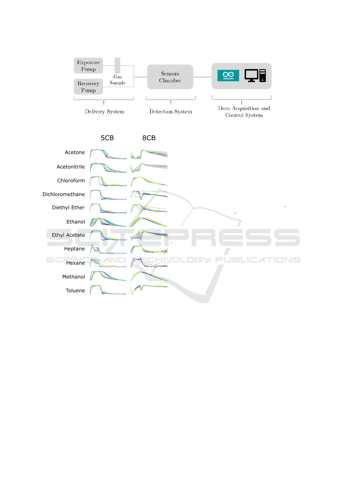
Figure 1: Schematic of the e-nose and its systems. Adapted from (Santos et al., 2019).

Figure 2: Representation of overlapped cycles obtained

with the optical sensing gels containing bovine gelatin

with the IL [BMIM][DCA] and LC 8CB, and the IL

[BMIM][DCA] and the LC 5CB for all VOCs.

problems is using a 1 NN-euclidean classiﬁer, which

works well with short signals, being also very quick.

In addition to this method, this work proposes a novel

methodology that intends to perform time series clas-

siﬁcation based on higher level structures with a lin-

guistic representation of the signals. The performance

of the latter will be compared with the standard 1 NN-

euclidean method.

3.1 Pre-processing

The analysis starts with a pre-processing stage, which

comprehends three main steps: (1) noise reduction,

(2) cycle segmentation and (3) outlier removal. The

ﬁrst step will be ﬁltering the signals by applying a

median ﬁlter and a smoothing function, to ensure high

frequency noise and high ﬂuctuations are attenuated.

The median ﬁlter has as input the signal and the size

of the median ﬁlter window, returning a signal with

the same size as the original containing the median

ﬁltered result. The smooth function uses a window

with 1 second.

The dataset for each experiment has a square sig-

nal that indicates the moments in which the pumps

are working, which are the exposure (pump signal =

1) and recovery (pump signal = 0). This information

was used to split the signals into individual cycles.

Cycles with a signal-to-noise ratio inferior to 3 are re-

moved, as well as outliers, identiﬁed by calculating

the euclidean distance of a cycle to the mean wave of

the experiment.

3.2 Time Series: Word Vector Classiﬁer

The proposed methodology is inspired by the reason-

ing from text data mining for text classiﬁcation. This

pipeline uses the well known Bag of Words (BoW)

to generate a feature matrix with vectors that repre-

sent the frequency of words found for each document.

Each vector is a representation of a document. From

this matrix, a simple classiﬁer such as a naive bayes

model or a linear Support Vector Machine (SVM) can

be used (HaCohen-Kerner et al., 2020). Besides, the

BoW matrix can be converted to a term-frequency in-

verse frequency (Tf-idf ) matrix as well. In order to

use this reasoning, the time series needs to be con-

verted to text, adding a ”sentence generation” layer to

the process. In this case, the conversion to text is per-

formed with SSTS, which applies a conversion of the

time series to text based on (1) a pre-processing step

and (2) a connotation step. Patterns are then found

in a third step (3) the search. For this, a regular ex-

pression is used in this symbolic representation, and

words are generated for each of the patterns found,

building a representation with written sentences.

The overall process is depicted in Figure 3.

Classiﬁcation of Volatile Compounds with Morphological Analysis of e-nose Response

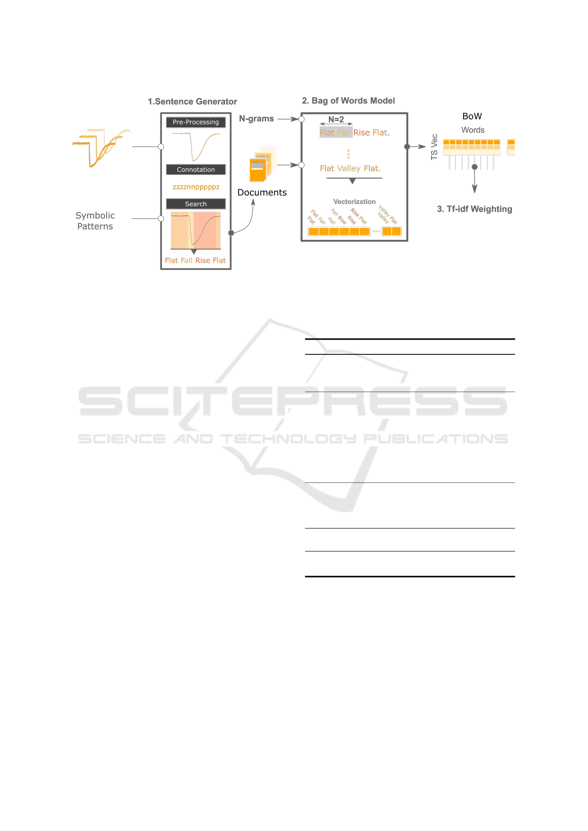
Figure 3: Steps for the vectorization of the set of time series to be classiﬁed. Step 1: Convert the time series into sentences;

Step 2: Convert the sentences into a vectorized representation (BoW); Step 3: Transform the BoW into the Tf-idf.

3.2.1 Pattern Search and Sentence Generation

As presented in Figure 3, the process starts by con-

verting the signal into a symbolic representation.

Each step of SSTS is selected by the user to opti-

mize the search of the desired pattern. For example,

when searching for moments when the signal is ris-

ing, the user selects (1) the pre-processing that best

can prepare the signal for this search, (2) the connota-

tion that corresponds to the ﬁrst derivative, converting

each sample of the signal into a character for when it

is rising (p), falling (n) or ﬂat (z). The rising mo-

ments of the signal are then searched with a regular

expression, such as ”p+”. To this pattern, the word

”Rise” is attributed. This process is applied for a pre-

deﬁned group of patterns and for each of these, a word

is given. The words are then ordered and the sentence

is build, as showed in step 1 of Figure 3.

The connotation methods used for this analysis

and the possible characters generated during this step

are presented in Table 1.

The list of patterns used for this analysis is pre-

sented in Table 2.

The pre-processing step is not presented in Table

1 as it is the same for all signals and made during the

pre-processing stage. The connotation and the search

step are showed and the corresponding word assigned

to the pattern as well. The groups of rows represent

the words that are used to build a sentence. As there

are 7 groups, in general, each signal is characterized

by 7 sentences. The search pattern is a regular ex-

pression that depends in the translation made by the

connotation method.

Table 1: Connotation (Con) methods and their meaning for

each single characters (Char) in which the samples of the

time series are translated.

Con Char Description

1st

Derivative

p positive slope

n negative slope

z zero slope

Slope

Height

r positive slope with low in-

crease

R positive slope with high in-

crease

f negative slope with low in-

crease

F negative slope with high in-

crease

Derivative

Speed

R quick positive slope

r slow positive slope

F quick negative slope

f slow negative slope

Amplitude

0 lower than a threshold

1 higher than a threshold

2nd

Derivative

D Concave

C Convex

3.2.2 Signal Vectorization

From the generated sentences, it is possible to use

natural language processing (NLP) techniques to per-

form a feature analysis and classiﬁcation. Typically,

the process involves using a BoW or a Tf-idf repre-

sentation, which are deﬁned by evaluating the num-

ber of occurrences of words in a document. For each

signal, a document and a corresponding vector, with

word occurrences (tf ), is generated for each signal.

This vector can be compared with the other vectors

BIOSIGNALS 2022 - 15th International Conference on Bio-inspired Systems and Signal Processing

Table 2: The connotation variables, search regular ex-

pressions and corresponding words assigned to the pattern

searched. The parameter m indicates the size, in samples, of

the difference between a peak or a plateau. For this work,

m=20 samples.

Connotation Search Word

Derivative

p+ Rising

n+ Falling

z+ Flat

Derivative

p+z{,m}n+ Peak

n+z{,m}p+ Valley

p+z{m,}n+ posPlateau

n+z{m,}p+ negPlateau

Slope

Height

r+ smallRise

R+ highRise

f+ smallFall

F+ highFall

Slope

Height

r+z*F+ smallRisehighFall

R+z*f+ highRisesmallFall

f+z*r+ smallFallsmallRise

F+z*R+ highFallhighRise

r+z*f+ smallRisesmallFall

R+z*F+ highRisehighFall

f+z*R+ smallFallhighRise

F+z*r+ highFallsmallRise

Derivative

Speed

R+ quickRise

r+ slowRise

F+ quickFall

r+ slowFall

z+ Straight

Ampltiude

Derivative

(0p)+(0z)*(0n)+ lowPeak

(1p)+(1z)*(1n)+ highPeak

(0n)+(0z)*(0p)+ lowValley

(1n)+(1z)*(1p)+ highValley

2nd

Deriva-

tive + 1st

Derivative

(Dp)+ concaveRising

(Dn)+ concaveFalling

(Cp)+ convexRising

(Cn)+ convexFalling

to evaluate the similarity between signals. The BoW

vectors are made with the following formula:

t f

t,d

∑

∈d

(1)

being t the word that exists in all documents, d the

document, t’ the term that belongs to document d.

As presented in Figure 3, in the step 2, the BoW is

built with the possibility of gaining context over what

surrounds the words in a sentence, for instance, if the

sequence ”Flat Rise” is common in one of the classes,

it might be an important feature, more than the indi-

vidual counterparts, ”Flat” and ”Rise”. In that sense,

an N-gram was given to build the BoW. In the exam-

ple presented, an N-gram of size 2 is used and the

ﬁnal example vector is generated from the sentences

of the document. From sentence ”Flat Valley Flat”,

the words ”Flat”, ”Valley”, ”Flat Valley” and ”Valley

Flat” are represented. For this work, an N-gram value

of 5 was used.

3.2.3 The Tf-idf Representation

Opposed to the BoW model, the Tf-idf model max-

imizes differences between documents by means of

including the inverse document frequency term (idf),

represented by the following equations:

id f (t, D) = log

|d ∈ D : t ∈ d|

(2)

being D, the set of documents and N the total number

of documents. The ﬁnal equation of the Tf-idf model

is the following:

t f id f (t, d, D) = t f (t, d) · id f (t, D) (3)

This matrix was the chosen representation, as the

literature emphasises that better results are typically

achieved and other methods that use symbolic repre-

sentation of time series use Tf-idf by default (Sch

afer,

2015; Lin et al., 2012). This model will be used with

a SVM with a linear kernel (linearSVC) for the VOC

classiﬁcation. The sklearn package from Python was

used to perform both vectorization and classiﬁcation

steps.

4 RESULTS AND DISCUSSION

The classiﬁcation of VOCs was performed with both

a 1-NN-euclidean classiﬁer and a novel proposed

method TSWordVectorizer. The results are presented

in Figures 4 and 5, respectively. These Figures show

the averaged confusion matrices for both methods

over using each experiment as a testing set. In ad-

dition, Table 3 show the overall performance of both

methods for both sensing formulations.

4.1 Ability to Classify VOCs

The results presented by Figures 4 and 5 show that the

e-nose is able to produce different signals for different

VOCs. The 5CB formulation was better in doing so,

providing better results for both methods. Regarding

the signals from the 5CB formulation, it is relevant to

mention that experiments acquired in different days

are able to be reproduced over time. Considering that

experimental conditions may vary due to slight differ-

ences in the VOC concentration, or in the preparation

of the formulation, the 5CB sensor is able to provide

signals that account for this variability. This was not

Classiﬁcation of Volatile Compounds with Morphological Analysis of e-nose Response

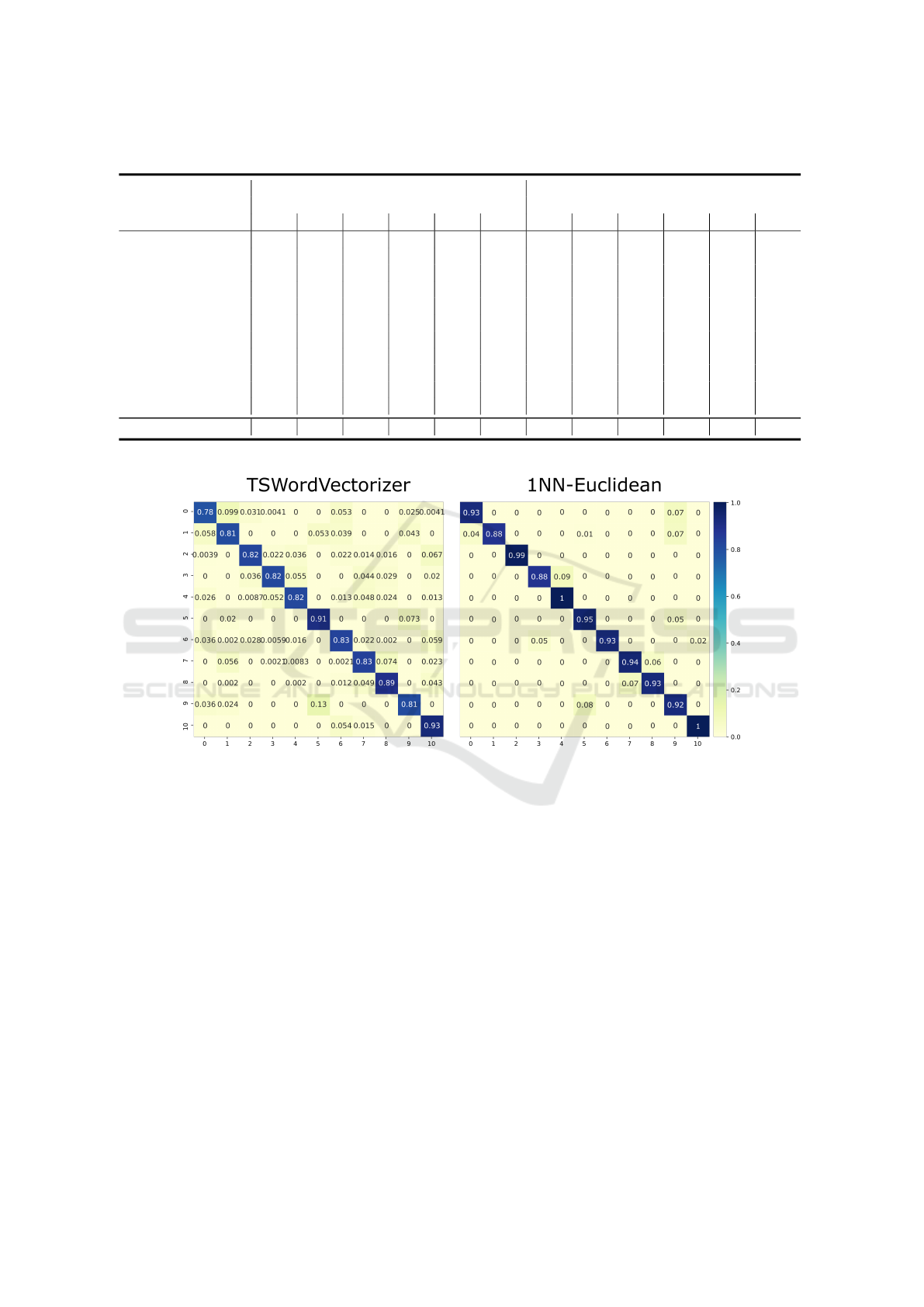
Table 3: Overall results of the classiﬁcation of VOCs for both used methods and both sensor formulations.

VOC

TSWordVectorizer 1 NN-euclidean

8CB 5CB 8CB 5CB

P R F1 P R F1 P R F1 P R F1

Acetone 0.76 0.94 0.84 0.83 0.78 0.80 0.77 0.83 0.80 0.95 0.93 0.94

Acetonitrile

0.84 0.82 0.83 0.81 0.81 0.81 0.65 1.00 0.79 1.00 0.88 0.94

Chloroform 0.94 0.90 0.92 0.89 0.82 0.85 1.00 1.00 1.00 1.00 0.99 0.99

Dicholoromethane 0.89 0.61 0.72 0.91 0.82 0.86 0.78 0.54 0.64 0.95 0.88 0.91

Diethyl Ether 0.87 0.84 0.86 0.86 0.82 0.84 0.62 0.83 0.71 0.91 1.00 0.95

Ethanol 0.61 0.60 0.61 0.82 0.91 0.86 0.85 0.79 0.81 0.92 0.95 0.93

Ethyl Acetate 0.85 0.67 0.75 0.81 0.83 0.82 1.00 0.75 0.80 0.98 0.93 0.95

Heptane 0.53 0.60 0.56 0.81 0.83 0.82 0.89 0.62 0.73 0.93 0.94 0.94

Hexane 0.51 0.40 0.45 0.86 0.89 0.87 0.80 0.73 0.76 0.94 0.93 0.94

Methanol 0.65 0.61 0.63 0.85 0.81 0.83 0.77 0.83 0.80 0.83 0.92 0.87

Toluene 0.66 0.91 0.77 0.80 0.93 0.86 1.00 1.00 1.00 0.94 1.00 0.97

Total 0.74 0.72 0.72 0.84 0.84 0.84 0.83 0.81 0.80 0.94 0.94 0.94

P - Precision; R - Recall; F1 - f1-score.

Figure 4: Confusion matrix of the classiﬁcation of VOCs with the 5CB formulation for both methods. An average f1-score of

84.0% and 94.0% was achieved for TSWordVectorizer and 1-NN-Euclidean methods, respectively. The analyzed VOCs are

labelled from 0 to 10 in the following order: acetone, acetonitrile, chloroform, dichloromethane, diethyl ether, ethanol, ethyl

acetate, heptane, hexane, methanol, and toluene.

met with the 8CB sensor. In this case, the signals gen-

erated are richer in their morphological changes, but

a higher variability in the shape of the signal is found

in different experiments. Even so, the fact that less

experiments were used with the 8CB sensor can in-

dicate that more experiments are needed to make the

database more robust.

Overall, the 5CB formulation was able to provide

better results than 8CB with both classiﬁcation meth-

ods.

4.2 Comparison between Methods

The TSWordVectorizer model shows to be promis-

ing in performing this type of tasks. Although rely-

ing solely in a higher structural level, describing the

morphological sequence based on the ordered pres-

ence of patterns, this method was able to mostly cor-

rectly classify each VOCs, with an average f1-score

of 84% for the 5CB formulation and 72% for the

8CB formulation. This method had more difﬁculties

in classifying VOCs that had very similar morphol-

ogy. For instance, the 8CB sensor exhibited a very

similar response to Ethanol and Methanol, as well

as to Heptane and Hexane (Figure 2). In that sense,

more mistakes are made between these compounds,

which is also veriﬁed with the euclidean method but

with less impact in the overall performance. The 1-

NN-euclidean method achieved an average f1-score

of 94.0% and 81.4% for the 5CB and 8CB formula-

tions, respectively.

BIOSIGNALS 2022 - 15th International Conference on Bio-inspired Systems and Signal Processing

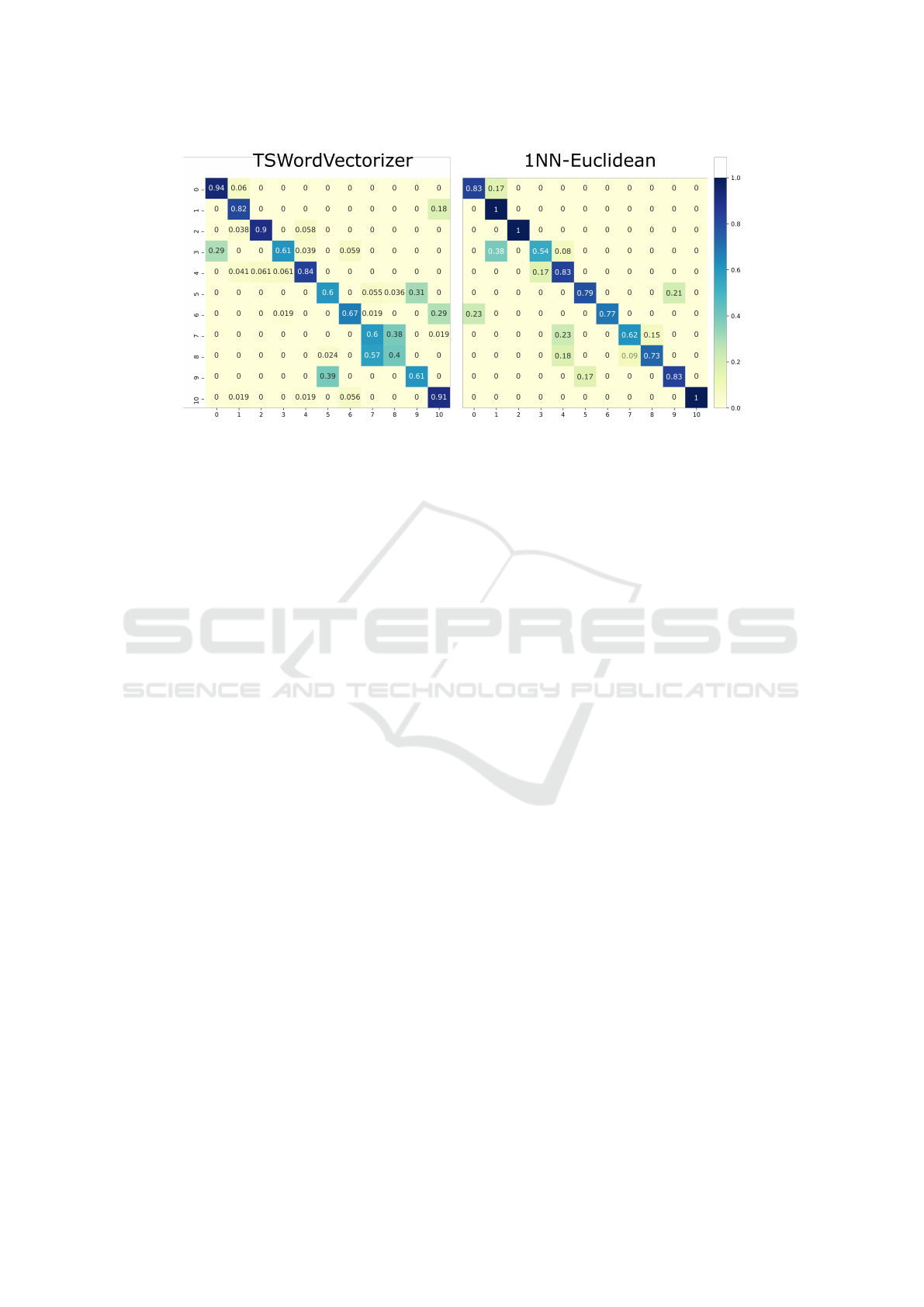
Figure 5: Confusion matrix of the classiﬁcation of VOCs with the 8CB formulation for both methods. An average f1-score of

72.0% and 81.4% was achieved for TSWordVectorizer and 1-NN-Euclidean methods, respectively. The analyzed VOCs are

labelled from 0 to 10 in the following order: acetone, acetonitrile, chloroform, dichloromethane, diethyl ether, ethanol, ethyl

acetate, heptane, hexane, methanol, and toluene.

Both methods follow the same tendency for each

VOC: the precision is higher or lower for the same

VOCs. Nevertheless, the TSWordVectorizer was not

as good as the simpler and quicker 1-NN-euclidean

method, which means that improvements have to be

made. In the literature, dictionary-based methods,

such as this one, are recommended for longer time

series, with higher structural differences. In order to

be applied successfully on short time series, other de-

scriptions have to be designed, reﬂecting the presence

of other patterns that can highlight other properties

of the signal. In addition, several classiﬁcation mis-

takes were made because the shape differences are not

at the overall shape level, but rather in the properties

of the shape itself. For instance, regarding Methanol

and Ethanol of formulation 8CB, the shape is exactly

the same, but differences in how the signal rises and

falls are what enable the distinction made by the eu-

clidean method. In that sense, another layer of analy-

sis could be added regarding the properties of the ex-

isting shapes, enabling the differentiation of signals

with the same overall shape. Moreover, a grid search

over the variables of the method should be performed

to optimize the performance, namely for the n-gram

value and peak size (m parameter in Table 2).

5 CONCLUSION AND FUTURE

WORK

The main purpose of this work was to discover if it

was possible to predict the label of a VOC by means

of a previous database acquired with the same e-nose

and sensors but with past samples of the same type

of VOC. This was achieved with excellent accuracy

for the 5CB formulation and medium accuracy for the

8CB formulation, using two different time series anal-

ysis methods. More data should be acquired to build

a robust database for the differentiation of such com-

pounds. The possibility of combining multiple for-

mulations in the same e-nose is also promising and

would deﬁnitely improve the performance.

The usage of a simple and standard method as the

1 NN-euclidean was good enough to perform a clear

identiﬁcation of the correct VOCs, which is promis-

ing, since the process is simple and quick. In the

other hand, the proposed method was not as good, but

shows promising results for this type of task. More

improvements should be made, namely in perform-

ing a differentiation at the feature level of the patterns

used to describe the signals. Additionally, more pat-

terns can be deﬁned to highlight other dynamics of the

signals. Besides, this method could be used with other

classiﬁers in an ensemble learning pipeline, since it

gives a different look over the signals.

Finally, the proposed methodology has the poten-

tial to deliver an explainability and interpretability

over the differences between classes, namely by us-

ing the Tf-idf weight values for each pattern (Senin

and Malinchik, 2013).

In this work, we have demonstrated the applica-

bility of TSWordVectorizer to VOC-sensing signals

in an innovative signal analysis pipeline that shows

potential for further improvements and expansion to

real-world VOC samples classiﬁcation.

Classiﬁcation of Volatile Compounds with Morphological Analysis of e-nose Response

ACKNOWLEDGEMENTS

This project has received funding from the European

Research Council (ERC) under the EU Horizon 2020

research and innovation programme [grant reference

SCENT-ERC-2014-STG-639123, (2015-2022)] and

by national funds from FCT - Fundac¸

ao para a

encia e a Tecnologia, I.P., in the scope of the

project UIDP/04378/2020 and UIDB/04378/2020 of

the Research Unit on Applied Molecular Biosciences

– UCIBIO and the project LA/P/0140/2020 of the As-

sociate Laboratory Institute for Health and Bioecon-

omy - i4HB, which is ﬁnanced by national funds from

ﬁnanced by FCT/MEC (UID/Multi/04378/2019).

This work was also partly supported by Fundac¸

para a Ci

encia e Tecnologia, under PhD grant

PD/BDE/142816/2018.

REFERENCES

Bos, L. D. J., Sterk, P. J., and Schultz, M. J. (2013).

Volatile Metabolites of Pathogens: A Systematic Re-

view. PLoS Pathogens, 9(5):e1003311.

Bruins, M., Rahim, Z., Bos, A., van de Sande, W. W., Endtz,

H. P., and van Belkum, A. (2013). Diagnosis of active

tuberculosis by e-nose analysis of exhaled air. Tuber-

culosis, 93(2):232–238.

Chandler, R., Das, A., Gibson, T., and Dutta, R. (2015). De-

tection of oil pollution in seawater: Biosecurity pre-

vention using electronic nose technology. In 2015 31st

IEEE International Conference on Data Engineering

Workshops, volume 2015-June, pages 98–100. IEEE.

Chen, L.-Y., Wong, D.-M., Fang, C.-Y., Chiu, C.-I., Chou,

T.-I., Wu, C.-C., Chiu, S.-W., and Tang, K.-T. (2018).

Development of an electronic-nose system for fruit

maturity and quality monitoring. In 2018 IEEE In-

ternational Conference on Applied System Invention

(ICASI), pages 1129–1130. IEEE.

Coronel Teixeira, R., Rodr

ıguez, M., Jim

enez de Romero,

N., Bruins, M., G

omez, R., Yntema, J. B., Cha-

parro Abente, G., Gerritsen, J. W., Wiegerinck, W.,

erez Bejerano, D., and Magis-Escurra, C. (2017).

The potential of a portable, point-of-care electronic

nose to diagnose tuberculosis. Journal of Infection,

75(5):441–447.

Di Natale, C., Macagnano, A., Martinelli, E., Paolesse, R.,

D’Arcangelo, G., Roscioni, C., Finazzi-Agr

o, A., and

D’Amico, A. (2003). Lung cancer identiﬁcation by

the analysis of breath by means of an array of non-

selective gas sensors. Biosensors and Bioelectronics,

18(10):1209–1218.

Esteves, C., Santos, G. M., Alves, C., Palma, S. I., Porteira,

A. R., Filho, J., Costa, H. M., Alves, V. D., Morais

Faustino, B. M., Ferreira, I., Gamboa, H., and Roque,

A. C. (2019). Effect of ﬁlm thickness in gelatin hy-

brid gels for artiﬁcial olfaction. Materials Today Bio,

1(December 2018):100002.

Fens, N., Zwinderman, A. H., van der Schee, M. P., de Nijs,

S. B., Dijkers, E., Roldaan, A. C., Cheung, D., Bel,

E. H., and Sterk, P. J. (2009). Exhaled Breath Pro-

ﬁling Enables Discrimination of Chronic Obstruc-

tive Pulmonary Disease and Asthma. American

Journal of Respiratory and Critical Care Medicine,

180(11):1076–1082.

Fraz

ao, J., Palma, S. I. C. J., Costa, H. M. A., Alves, C.,

Roque, A. C. A., and Silveira, M. (2021). Optical Gas

Sensing with Liquid Crystal Droplets and Convolu-

tional Neural Networks. Sensors, 21(8):2854.

HaCohen-Kerner, Y., Miller, D., and Yigal, Y. (2020). The

inﬂuence of preprocessing on text classiﬁcation using

a bag-of-words representation. PLOS ONE, 15(5):1–

22.

Hockstein, N. G., Thaler, E. R., Lin, Y., Lee, D. D., and

Hanson, C. W. (2005). Correlation of Pneumonia

Score with Electronic Nose Signature: A Prospective

Study. Annals of Otology, Rhinology & Laryngology,

114(7):504–508.

Hockstein, N. G., Thaler, E. R., Torigian, D., Miller,

W. T., Deffenderfer, O., and Hanson, C. W. (2004).

Diagnosis of Pneumonia With an Electronic Nose:

Correlation of Vapor Signature With Chest Com-

puted Tomography Scan Findings. The Laryngoscope,

114(10):1701–1705.

Hu, W., Wan, L., Jian, Y., Ren, C., Jin, K., Su, X., Bai, X.,

Haick, H., Yao, M., and Wu, W. (2018). Electronic

Noses: From Advanced Materials to Sensors Aided

with Data Processing. Advanced Materials Technolo-

gies, 4(2):1–38.

Hussain, A., Semeano, A. T. S., Palma, S. I. C. J., Pina,

A. S., Almeida, J., Medrado, B. F., P

adua, A. C.

C. S., Carvalho, A. L., Dion

ısio, M., Li, R. W. C.,

Gamboa, H., Ulijn, R. V., Gruber, J., and Roque, A.

C. A. (2017). Tunable Gas Sensing Gels by Coop-

erative Assembly. Advanced Functional Materials,

27(27):1700803.

Karakaya, D., Ulucan, O., and Turkan, M. (2020). Elec-

tronic Nose and Its Applications: A Survey. In-

ternational Journal of Automation and Computing,

17(2):179–209.

Keogh, E., Lonardi, S., and Ratanamahatana, C. A. (2004).

Towards parameter-free data mining. In Proceedings

of the Tenth ACM SIGKDD International Conference

on Knowledge Discovery and Data Mining, KDD ’04,

page 206–215, New York, NY, USA. Association for

Computing Machinery.

Lee, Y.-S., Joo, B.-S., Choi, N.-J., Lim, J.-O., Huh, J.-S.,

and Lee, D.-D. (2003). Visible optical sensing of am-

monia based on polyaniline ﬁlm. Sensors and Actua-

tors B: Chemical, 93(1-3):148–152.

Lin, J., Keogh, E., Wei, L., and Lonardi, S. (2007). Expe-

riencing sax: A novel symbolic representation of time

series. Data Min. Knowl. Discov., 15:107–144.

Lin, J., Khade, R., and Li, Y. (2012). Rotation-invariant

similarity in time series using bag-of-patterns repre-

sentation. J. Intell. Inf. Syst., 39(2):287–315.

adua, A. C., Palma, S., Gruber, J., Gamboa, H., and

Roque, A. C. (2018). Design and evolution of an opto-

electronic device for VOCs detection. BIODEVICES

BIOSIGNALS 2022 - 15th International Conference on Bio-inspired Systems and Signal Processing

2018 - 11th International Conference on Biomedical

Electronics and Devices, Proceedings; Part of 11th

International Joint Conference on Biomedical Engi-

neering Systems and Technologies, BIOSTEC 2018,

1(Biostec):48–55.

Pavlou, A. K., Magan, N., Jones, J. M., Brown, J., Klatser,

P., and Turner, A. P. (2004). Detection of Mycobac-

terium tuberculosis (TB) in vitro and in situ using an

electronic nose in combination with a neural network

system. Biosensors and Bioelectronics, 20(3):538–

544.

Persaud, K. and Dodd, G. (1982). Analysis of discrimina-

tion mechanisms in the mammalian olfactory system

using a model nose. Nature, 299(5881):352–355.

Saidi, T., Zaim, O., Mouﬁd, M., El Bari, N., Ionescu, R.,

and Bouchikhi, B. (2018). Exhaled breath analysis

using electronic nose and gas chromatography–mass

spectrometry for non-invasive diagnosis of chronic

kidney disease, diabetes mellitus and healthy subjects.

Sensors and Actuators, B: Chemical, 257:178–188.

Santos, G., Alves, C., P

adua, A., Palma, S., Gamboa, H.,

and Roque, A. (2019). An Optimized E-nose for Ef-

ﬁcient Volatile Sensing and Discrimination. In Pro-

ceedings of the 12th International Joint Conference on

Biomedical Engineering Systems and Technologies,

pages 36–46. SCITEPRESS - Science and Technol-

ogy Publications.

Santos, J., Garc

ıa, M., Aleixandre, M., Horrillo, M.,

Guti

errez, J., Sayago, I., Fern

andez, M., and Ar

es, L.

(2004). Electronic nose for the identiﬁcation of pig

feeding and ripening time in Iberian hams. Meat Sci-

ence, 66(3):727–732.

Sch

afer, P. (2015). The boss is concerned with time series

classiﬁcation in the presence of noise. Data Mining

Knowledge Discovery, 29(6):1505–1530.

Sch

afer, P. and Leser, U. (2017). Fast and Accurate Time Se-

ries Classiﬁcation with WEASEL, page 637–646. As-

sociation for Computing Machinery, New York, NY,

USA.

Senin, P. and Malinchik, S. (2013). Sax-vsm: Interpretable

time series classiﬁcation using sax and vector space

model.

Wilson, A. D. and Baietto, M. (2011). Advances

in Electronic-Nose Technologies Developed for

Biomedical Applications. Sensors, 11(1):1105–1176.

Classiﬁcation of Volatile Compounds with Morphological Analysis of e-nose Response