SDR-NNP: Sharpened Dimensionality Reduction with Neural Networks

Youngjoo Kim

1,† a

, Mateus Espadoto

2,† b

, Scott C. Trager

3 c

, Jos B. T. M. Roerdink

1 d

and

Alexandru C. Telea

4 e

Bernoulli Institute for Mathematics, Computer Science and Artiﬁcial Intelligence,

University of Groningen, The Netherlands

Institute of Mathematics and Statistics, University of S

ao Paulo, Brazil

Kapteyn Astronomical Institute, University of Groningen, The Netherlands

Department of Information and Computing Sciences, Utrecht University, The Netherlands

Keywords:

High-dimensional Visualization, Dimensionality Reduction, Mean Shift, Neural Networks.

Abstract:

Dimensionality reduction (DR) methods aim to map high-dimensional datasets to 2D scatterplots for visual

exploration. Such scatterplots are used to reason about the cluster structure of the data, so creating well-

separated visual clusters from existing data clusters is an important requirement of DR methods. Many DR

methods excel in speed, implementation simplicity, ease of use, stability, and out-of-sample capabilities, but

produce suboptimal cluster separation. Recently, Sharpened DR (SDR) was proposed to generically help such

methods by sharpening the data-distribution prior to the DR step. However, SDR has prohibitive computa-

tional costs for large datasets. We present SDR-NNP, a method that uses deep learning to keep the attractive

sharpening property of SDR while making it scalable, easy to use, and having the out-of-sample ability. We

demonstrate SDR-NNP on seven datasets, applied on three DR methods, using an extensive exploration of its

parameter space. Our results show that SDR-NNP consistently produces projections with clear cluster sepa-

ration, assessed both visually and by four quality metrics, at a fraction of the computational cost of SDR. We

show the added value of SDR-NNP in a concrete use-case involving the labeling of astronomical data.

1 INTRODUCTION

The visual analysis of high-dimensional data is chal-

lenging, due to its many observations (also known

as points or samples) and values recorded per obser-

vation (also known as dimensions, features, or vari-

ables) (Liu et al., 2015; Nonato and Aupetit, 2018;

Espadoto et al., 2019). Dimensionality reduction

(DR), also called projection, is particularly suited

for such data. Compared to glyphs (Yates et al.,

2014), parallel coordinate plots (Inselberg and Dims-

dale, 1990), table lenses (Rao and Card, 1994), and

scatterplot matrices (Becker et al., 1996), DR meth-

ods scale visually up to thousands of dimensions

and hundreds of thousands of samples. DR tech-

niques such as t-SNE (Maaten and Hinton, 2008) and

https://orcid.org/0000-0002-9677-163X

https://orcid.org/0000-0002-1922-4309

https://orcid.org/0000-0001-6994-3566

https://orcid.org/0000-0003-1092-9633

https://orcid.org/0000-0003-0750-0502

†

These authors contributed equally.

UMAP (McInnes and Healy, 2018), to mention the

most popular ones, can segregate data clusters into

well-separated visual clusters, which enables one to

reason about the former by seeing the latter, a prop-

erty generically known as preservation of data struc-

ture (Behrisch et al., 2018).

A recent survey (Espadoto et al., 2019) noted that

many DR techniques score below t-SNE or UMAP

in cluster segregation but have other assets – simple

usage and implementation, computational scalability,

and out-of-sample behavior. Following this, (Kim

et al., 2021) recently proposed Sharpened DR (SDR)

to generically improve the cluster segregation ability

by sharpening the data prior to DR by a variant of the

Mean Shift algorithm (Comaniciu and Meer, 2002).

However, SDR is impractical to use as Mean Shift

is prohibitively expensive in high dimensions. Sep-

arately, Neural Network Projection (NNP) was pro-

posed (Espadoto et al., 2020) to generically imitate

any DR technique with good quality, speed, ease-of-

use, and out-of-sample ability.

In this paper, we combine the cluster segregation

Kim, Y., Espadoto, M., Trager, S., Roerdink, J. and Telea, A.

SDR-NNP: Sharpened Dimensionality Reduction with Neural Networks.

DOI: 10.5220/0010820900003124

In Proceedings of the 17th International Joint Conference on Computer Vision, Imaging and Computer Graphics Theory and Applications (VISIGRAPP 2022) - Volume 3: IVAPP, pages 63-76

ISBN: 978-989-758-555-5; ISSN: 2184-4321

abilities of SDR with the speed, ease-of-use, and out-

of-sample abilities of NNP. Our approach jointly ad-

dresses the Mean Shift sharpening step of SDR and

the generic projection step following afterwards. Our

SDR-NNP method has the following features – to our

knowledge, not yet jointly achieved by existing DR

methods:

Quality (C1): We provide better cluster separation

than existing DR methods, as measured by well-

known metrics in the DR literature;

Scalability (C2): Our method is linear in sample and

dimension counts, allowing the projection of datasets

of up to a million samples and hundreds of dimen-

sions in a few seconds on commodity GPU hardware;

Ease of use (C3): Our method produces good results

with minimal or no parameter tuning;

Genericity (C4): We can handle any real-valued (un-

labeled) high-dimensional data;

Stability and Out-of-Sample Support (C5): We can

project new samples for a learned projection without

recomputing it, in contrast to standard t-SNE and any

other non-parametric methods.

We structure this paper as follows: Section 2 dis-

cusses related work on dimensionality reduction. Sec-

tion 3 details our method. Section 4 presents the re-

sults that support our above contributions. Section 5

discusses our method. Finally, Section 6 concludes

the paper.

2 BACKGROUND

Let x = (x

,. .. ,x

), x

∈ R,1 ≤ i ≤ n be an n-

dimensional (nD) real-valued sample, and let D =

}, 1 ≤ j ≤ N be a dataset of N samples. A DR

technique is a function

P : R

→ R

, (1)

where q  n, and typically q = 2. The projection P(x)

of a sample x ∈ D is a point p ∈ R

. Projecting the

whole set D yields a qD scatterplot denoted next as

P(D).

DR methods aim to satisfy multiple requirements.

Table 1 outlines prominent ones present in several

DR surveys (Hoffman and Grinstein, 2002; Maaten

and Postma, 2009; Engel et al., 2012; Sorzano et al.,

2014; Liu et al., 2015; Cunningham and Ghahramani,

2015; Xie et al., 2017; Nonato and Aupetit, 2018; Es-

padoto et al., 2019). Besides these, DR techniques

also require locality, steerability, and multilevel com-

putation (Nonato and Aupetit, 2018). We do not fo-

cus on such additional requirements as these are less

mainstream.

The quality (Q) and cluster separation (CS) re-

quirements need additional explanations. Projection

quality is assessed by local metrics that measure how

a small neighborhood of points in D maps to a neigh-

borhood in P(D) and/or conversely. Local quality

metrics include the following (see Table 2 for the for-

mal deﬁnitions):

Trustworthiness T (Venna and Kaski, 2006): Mea-

sures the fraction of close points in D that are also

close in P(D). T tells how much one can trust that lo-

cal patterns in a projection represent actual data pat-

terns. In the deﬁnition (Table 2), U

(K)

is the set of

points that are among the K nearest neighbors of point

i in the 2D space but not among the K nearest neigh-

bors of point i in R

; and r(i, j) is the rank of the 2D

point j in the ordered-set of nearest neighbors of i in

P(D);

Continuity C (Venna and Kaski, 2006): Measures

the fraction of close points in P(D) that are also close

in D. In the deﬁnition (Table 2), V

(K)

are the points in

the K nearest neighbors of point i in D but not among

the K nearest neighbors in 2D; and ˆr(i, j) is the rank of

the R

point j in the ordered set of nearest neighbors

of i in D;

Neighborhood Hit NH (Paulovich et al., 2008):

Measures how well a projection P(D) separates la-

beled data, in a rotation-invariant fashion. NH is

the number y

of the k nearest neighbors of a point

y ∈ P(D), denoted by y

, that have the same label l as

y, averaged over P(D);

Shepard Diagram Correlation R (Joia et al., 2011):

The Shepard diagram is a scatterplot of the pairwise

distances between all points in P(D) vs the corre-

sponding distances in D. Points below, respectively

above, the main diagonal show distance ranges for

which false neighbors, respectively missing neigh-

bors, occur. The closer the plot is to the main diag-

onal, the better the overall distance preservation is.

The scatterplot’s Spearman rank correlation R mea-

sures this – a value R = 1 indicates a perfect (positive)

distance correlation.

All above metrics are local, i.e., capture preserva-

tion of data structure in D at the scale given by the

neighborhood size K. In practice, what a ‘good’ K

value is for a given dataset D is unknown. K can also

vary locally within D as function of the point density.

At a higher level, projections are used to reason about

the overall data structure in D by creating, ideally, vi-

sual clusters that are as well separated in P(D) as data

clusters are in D, a property called cluster separa-

tion (CS). High-CS projections show, e.g., how many

point clusters exist and how these correlate (or not)

with labels or speciﬁc attributes (Nonato and Aupetit,

IVAPP 2022 - 13th International Conference on Information Visualization Theory and Applications

2018), or predict how easy it is to train a classiﬁer for

D based on the CS in P(D) (Rauber et al., 2017). In

general, it is hard to design objective metrics for CS

like one does for local quality, because a ‘well sepa-

rated data cluster’ in D is not evident. Hence, CS is

typically assessed on (labeled) datasets D for which

the ground-truth data-separation is well known, e.g.,

MNIST (LeCun and Cortes, 2010).

We next discuss existing DR methods in the light

of the requirements in Tab. 1. We group these into

unsupervised and supervised methods, as follows.

Unsupervised Methods: Principal Component Anal-

ysis (Jolliffe, 1986) (PCA) is simple, fast, out-of-

sample (OOS), and easy-to-interpret, also used as

pre-processing for other DR techniques that require a

moderate data dimensionality n (Nonato and Aupetit,

2018). Being a linear and global method, PCA is de-

ﬁcient on quality and CS, especially for data of high

intrinsic dimensionality.

Techniques such as MDS (Torgerson, 1958),

Landmark MDS (De Silva and Tenenbaum, 2004),

Isomap (Tenenbaum et al., 2000), and LLE (Roweis

and Saul, 2000) with its variations (Donoho and

Grimes, 2003; Zhang and Zha, 2004; Zhang and

Wang, 2007) detect and project the (neighborhood

of the) high-dimensional manifold on which data is

embedded, and can capture nonlinear data structure.

Such methods yield higher quality than PCA, but can

be hard to tune, do not all support OOS, and do not

work well for high-intrinsic-dimensional data.

Force-directed methods such as LAMP (Joia et al.,

2011) and LSP (Paulovich et al., 2008) can yield

good quality, good scalability, and are simple to

use. However, not all force-directed methods have

OOS capability. Clustering-based methods, such as

PBC (Paulovich and Minghim, 2006), share many

features with force-directed methods, such as good

quality, but also lack OOS.

Stochastic Neighborhood Embedding (SNE)

methods, like the well-known t-SNE (Maaten and

Hinton, 2008), have high overall quality and CS

capabilities. Yet, t-SNE has a (high) complexity of

O(N

) in sample count, is very sensitive to small data

changes, can be hard to tune (Wattenberg, 2016), and

has no OOS. Tree-accelerated t-SNE (Maaten, 2014),

hierarchical SNE (Pezzotti et al., 2016), approxi-

mated t-SNE (Pezzotti et al., 2017), and various GPU

variants of t-SNE (Pezzotti et al., 2020; Chan et al.,

2018) improve scalability, but are algorithmically

quite complex, and still have sensitivity, tuning, and

OOS issues. Uniform Manifold Approximation and

Projection (UMAP) (McInnes and Healy, 2018) has

comparable quality to t-SNE, is much faster and has

OOS. Still, UMAP is also sensitive to parameter

tuning.

Autoencoders (AE) (Hinton and Salakhutdinov,

2006; Kingma and Welling, 2013) aim to generate

a compressed, low-dimensional representation of the

data in their bottleneck layers by training to repro-

duce the data input at the output. They have similar

quality to PCA and are easy to set up, train, and use,

are fast, and have OOS capabilities. Self-organizing

maps (SOM) (Kohonen, 1997) share with AE the ease

of use, training, and computational scalability. Yet,

both AE and SOM lag behind t-SNE and UMAP in

CS, which is, as explained, essential for interpreting

projections.

Supervised Methods: ReNDA (Becker et al., 2020)

uses two neural networks to implement (1) a nonlinear

generalization of Fisher’s Linear Discriminant Anal-

ysis (Fisher, 1936) and (2) an autoencoder, used for

regularization. ReNDA scores well on predictability

and has OOS, but needs pre-training of each individ-

ual network and has low scalability. Recently, (Es-

padoto et al., 2020) proposed Neural Network Projec-

tions (NNP), where a selected subset D

⊂ D is pro-

jected by any DR method to yield a training projec-

tion P(D

) ⊂ R

. D

is fed into a regression neural

network which is trained to output a 2D scatterplot

that aims to replicate P(D

). NNP is very fast, simple

to use, generic, and has OOS. NNP’s major limitation

is a lower CS than its training projection.

Semi-supervised Methods: The SSNP

method (Espadoto et al., 2021) takes a mid path

between supervised methods (e.g., NNP) and unsu-

pervised ones (e.g., AE). Like NNP, SSNP has an

encoder-decoder architecture with a reconstruction

target but adds a classiﬁcation target using either

ground-truth labels from the dataset D or pseudola-

bels computed from D by a clustering algorithm.

SSNP produces 2D projections which look quite

similar to those created by our method described next

in Sec. 3. However, important differences exist:

• Our method consists of two distinct operations:

high-dimensional data sharpening, followed by

projection. SSNP only performs the projection

step;

• SSNP is a semi-supervised method that relies

upon labels or clustering to create the information

to learn from. Our method, similar to NNP, uses a

t-SNE projection of the data to learn from. This is

a fundamental difference between SSNP and our

method;

• The architectures of the neural networks for SSNP

and our method are fundamentally different. In

particular, SSNP uses two different architectures

for training, respectively inference. Our method

SDR-NNP: Sharpened Dimensionality Reduction with Neural Networks

Table 1: Summary of desirable requirements (characteristics) of DR methods.

Requirement name Description (the requirement implies that the method has the following properties):

Quality (Q) Captures local data structures well, as measured by the projection local-quality metrics in Table 2.

Cluster separation (CS) Captures data structures present at larger scales than local structures, e.g. clusters, as visual clusters in the 2D scatterplot.

Scalability (S) Can project datasets of hundreds of dimensions and millions of samples in a few seconds on commodity hardware.

Ease of use (EoU) Has few (ideally: no) free parameters, which are intuitive and easy to tune to get the desired results.

Genericity (G) Can project any (real-valued) dataset, with or without labels.

Out-of-sample (OOS) Can ﬁt new data in an existing projection. OOS projections are also stable – small input-data changes cause only small projection

changes.

Table 2: Local quality metrics for projections. All metrics range in [0,1] with 0 being lowest, and 1 being highest, quality.

Metric Deﬁnition

Trustworthiness (T ) 1 −

NK(2n−3K−1)

∑

i=1

∑

j∈U

(K)

(r(i, j) −K)

Continuity (C) 1 −

NK(2n−3K−1)

∑

i=1

∑

j∈V

(K)

(ˆr(i, j) −K)

Neighborhood hit (NH)

∑

y∈P(D)

Shepard diagram correlation (R) Spearman’s rank of (kx

− x

k,kP(x

) − P(x

)k),1 ≤ i ≤ N,i 6= j

uses a single architecture for both training and in-

ference.

• A key underlying use-case for SDR-NNP is to en-

hance the separation between unlabeled data clus-

ters so that these can next be labeled by users (see

next Sec. 4.3). This is out of scope of SSNP.

Sharpening Data: Finding clusters of related data

points is a key task in data science, addressed by

tens of clustering methods (Xu and Wunsch, 2005;

Berkhin, 2006). Mean Shift (MS) (Fukunaga and

Hostetler, 1975; Cheng, 1995; Comaniciu and Meer,

2002) is particularly relevant to our work. MS com-

putes the kernel density estimation of a dataset D and

next shifts points in D upstream along the density gra-

dient. This effectively clusters D, with applications in

image segmentation (Comaniciu and Meer, 2002) and

graph drawing (Hurter et al., 2012). Recently, Sharp-

ened DR (SDR) (Kim et al., 2021) used MS for the

ﬁrst time to assist DR: A dataset D is sharpened by a

few MS iterations, not to be confused with the clus-

tering goal of the original MS. The sharpened dataset

is next projected by a fast, easy-to-use, stable, but po-

tentially low-CS DR method. Sharpening ‘precondi-

tions’ the used DR method to overcome its lack of CS.

Yet, as MS is very slow for high-dimensional data,

this makes SDR impractical for such data.

Table 3 summarizes the DR techniques discussed

above and indicates how they fare with respect to the

requirements discussed earlier in this section. No

reviewed method satisﬁes all the requirements opti-

mally. We next describe our proposed method SDR-

NNP (Table 3 last row) and show that it scores high

on these requirements.

3 SDR-NNP METHOD

As outlined in Sec. 2, SDR and NNP have comple-

mentary desirable features: SDR produces good clus-

Table 3: Summary of DR techniques in Sec. 2 and their

characteristics from Table 1.

Desirable characteristics of the method

Method Q S EoU G OOS

PCA low high high high yes

MDS mid low low low no

L-MDS mid mid low low no

Isomap mid low low low no

LLE mid low low low no

LAMP mid mid mid high yes

LSP mid mid mid high no

PBC mid mid mid high no

UMAP high high low high yes

t-SNE high low low high no

Autoencoder low high high low yes

SOM low high high low no

ReNDA mid low low mid yes

NNP high high high high yes

SDR high low mid high no

SDR-NNP high high high high yes

ter separation (CS), while NNP is fast, easy to use,

and has OOS ability. Our combined SDR-NNP tech-

nique joins these advantages and works as follows

(see also Fig. 1). We use SDR to sharpen a small data

subset to create an initial 2D projection (Sec. 3.1).

Next, we train NNP on the sharpened data and its 2D

projection (Sec. 3.2) and use it to project the whole

dataset.

3.1 Sharpened Dimensionality

Reduction

SDR has two main components, as follows (for full

details we refer to (Kim et al., 2021)):

Sharpening the Data: Given a dataset D ∈ R

, SDR

computes its density using the multivariate kernel

density estimator ρ(x) : R

→ R

deﬁned as

ρ(x) =

∑

y∈N(x)



kx − yk



, (2)

where N(x) is the set of k

-nearest neighbors of x in

IVAPP 2022 - 13th International Conference on Information Visualization Theory and Applications

D; L is a parabolic kernel (Epanechnikov, 1969); and

h is the distance of x to its k

(farthest) neighbor in

N(x).

Next, SDR shifts points x ∈ D using the update

rule

= x + α

∇ρ(x)

max(k∇ρ(x)k,ε)

, (3)

where α ∈ [0,1] is a ‘learning rate’ parameter that

controls the shift speed (higher values yield higher

speed) and ε = 10

−5

is a regularization parameter.

After every update (Eqn. 3), the density ρ is com-

puted again using Eqn. 2. This sharpening approach

is called Local Gradient Clustering (LGC) by anal-

ogy with Gradient Clustering (GC) (Fukunaga and

Hostetler, 1975).

SDR has three parameters: T (number of itera-

tions); k

(number of nearest neighbors); and α (learn-

ing rate). We use k

≥ 50 following (Kim et al., 2021);

setting α and T is discussed in Sec. 4.

Projection: SDR produces a dataset D

which is a

sharpened version of the input dataset D. SDR next

projects D

by a DR method of choice (typically fast

but not necessarily OOS), called the baseline DR

method below, to obtain a 2D projection P(D

). The

data in D

are better separated than in D, which allows

a projection P to produce better cluster separation in

P(D

) than in P(D).

3.2 Training NNP

The key idea of SDR-NNP is to use SDR (Sec. 3.1) on

a small data subset to obtain P(D

). To project the full

dataset D, we next train the NNP regressor (Espadoto

et al., 2020) using D

as the high-dimensional in-

put and P(D

) as the 2D output. The network has

three fully-connected hidden layers with ReLU acti-

vation (Agarap, 2018), initial weights set to He Uni-

form (He et al., 2015), and an initial bias value set to

0.0001. The output layer has 2 units, one per 2D co-

ordinate, and uses sigmoid activation to constrain out-

put values to [0,1]. We used three different network

sizes, namely, x-small (75, 30, 75 units per layer),

small (150, 60, 150 units per layer) and medium (300,

120, 300 units per layer). We trained the network us-

ing the ADAM optimizer (Kingma and Ba, 2014), as

described in the NNP paper.

Figure 1: Architecture of the SDR-NNP pipeline.

After training, we have a regressor able to mimic

the behavior of SDR for unseen data, thus adding sta-

bility, OOS capability, and computational scalability

to SDR.

4 RESULTS

We measured the performance of SDR-NNP by the

four metrics in Tab. 2 computed for K = 7, in line

with (Maaten and Postma, 2009; Martins et al., 2015;

Espadoto et al., 2019). Note that K, the number

of nearest neighbors used to compute the metrics in

Tab. 2, is smaller than k

, the number of nearest met-

rics used to evaluate L (Eqn. 2). Indeed, k

needs to be

relatively large to smooth out local noise in the com-

putation of the gradient ∇ρ; in contrast, K is typically

set small to capture more local quality aspects of a

projection.

Evaluation used six publicly available real-

world datasets (Table 4), all being reasonably high-

dimensional and large (tens of dimensions, thousands

of samples), and with a non-trivial data structure. All

dimensions were rescaled to the [0,1] range, to match

NNP’s sigmoid activation function used in its output

layer (Sec. 3). All computed metrics can be found in

the Appendix.

Section 4.1 details the quality of SDR-NNP

trained to mimic SDR in combination with Landmark

MDS (LMDS), PCA, and t-SNE. Section 4.2 studies

the computational scalability of SDR-NNP. Finally,

Section 4.3 presents an application of SDR-NNP to

the analysis of an astronomical dataset.

4.1 Quality on Real-world Datasets

We studied SDR-NNP’s quality with respect to its

parameters (number of iterations T , learning rate α,

training epochs E, and NNP network size) using

LMDS, t-SNE, and PCA as baseline DR methods. A

discussion on the selection of DR methods for SDR

can be found in Sec. 6 from (Kim et al., 2021). For

space reasons we omitted results for all network sizes

other than medium.

Figure 2 shows how the number of iterations T

affects the sharpening of clusters for LMDS and t-

SNE (PCA results omitted for space reasons). For all

datasets, 4 to 8 iterations sufﬁce to have the clusters

sharply deﬁned in the projection. Table 7 in the Ap-

pendix shows quality metrics as functions of T for all

three baseline projections. Increasing T can increase

quality (Air Quality, Reuters with LMDS and PCA)

but generally slightly decreases quality for LMDS

and PCA. For t-SNE, this decrease is visible for all

SDR-NNP: Sharpened Dimensionality Reduction with Neural Networks

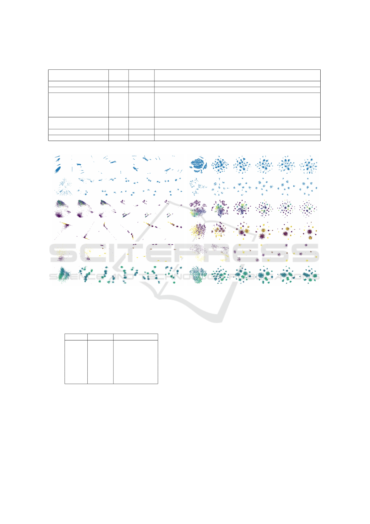
Table 4: Datasets used in SDR-NNP’s evaluation.

Dataset name Samples Dimensions Data description

and provenance N n

Air Quality (Vito et al., 2008) 9358 13 Measurements from air sensors used to study and predict air quality

Concrete (Yeh, 1998) 1030 8 Measurements of chemico-physical properties of concrete used to study concrete strength

Reuters (Thoma, 2017) 5000 100 Attributes extracted from news report documents using TF-IDF (Salton and McGill, 1986),

a standard method in text processing. This is a subset of the full dataset which contains data

for the six most frequent classes only. Used to study how features can predict news’ types

(classes)

Spambase (Hopkins et al.,

1999)

4001 57 Text dataset used to train email spam classiﬁers

Wisconsin (Street et al., 1993) 569 32 Features extracted from images of breast masses used to detect malignant cells

Wine (Cortez et al., 2009) 6497 11 Samples of white and red Portuguese vinho verde used to describe perceived wine quality

No SDR 4 iters 8 iters 12 iters 16 iters 20 iters

Wine Wisconsin Spambase Reuters Concrete Air Quality

(a) LMDS.

No SDR 4 iters 8 iters 12 iters 16 iters 20 iters

Wine Wisconsin Spambase Reuters Concrete Air Quality

(b) t-SNE.

Figure 2: Iteration parameter effect: SDR-NNP learned from LMDS (a) and t-SNE (b) for varying iterations T (columns) and

datasets (rows). Fixed SDR-NNP parameters are α = 0.1, E = 1000 epochs, medium network size.

Table 5: Time measurements for SDR and SDR-NNP (sec-

onds), GALAH dataset. See also Fig. 6.

Samples SDR SDR-NNP inference

1000 0.220 0.108

2000 0.957 0.059

5000 14.799 0.092

10000 157.420 0.149

20000 1302.268 0.414

30000 4736.995 0.355

40000 11058.267 0.727

datasets, which is explainable by the fact that t-SNE

already has a very high quality which is hard to be

learned by NNP (see (Espadoto et al., 2020)). How-

ever, as already argued in (Kim et al., 2021), local

quality metrics will likely decrease when using SDR

to favor visual cluster separation.

Figure 3 shows results for SDR-NNP when vary-

ing the learning rate α for LMDS and t-SNE (PCA

results omitted again for space reasons). Too small

or too large α values tend to affect the scatterplot ad-

versely. Values in the range α ∈ [0.05, 0.1] show the

best results, i.e., a good separation of the projection

into distinct clusters. Table 8 in the Appendix shows

quality metrics as function of α for all three base-

line projections. The effect of α on quality is similar

with that of T with some combinations (Reuters with

LMDS and PCA) showing a slight increase but most

showing a slight decrease for small α values.

Figure 4 shows how the number of training epochs

E affects projection quality. The early stopping strat-

egy proposed in the NNP paper (Espadoto et al.,

2020), which stops training on convergence, deﬁned

as the epoch where the validation loss stops decreas-

ing (roughly E = 60 epochs in practice), does not pro-

duce good results for SDR-NNP – the resulting pro-

jection (Fig. 4a,b leftmost columns) show a fuzzy ver-

IVAPP 2022 - 13th International Conference on Information Visualization Theory and Applications

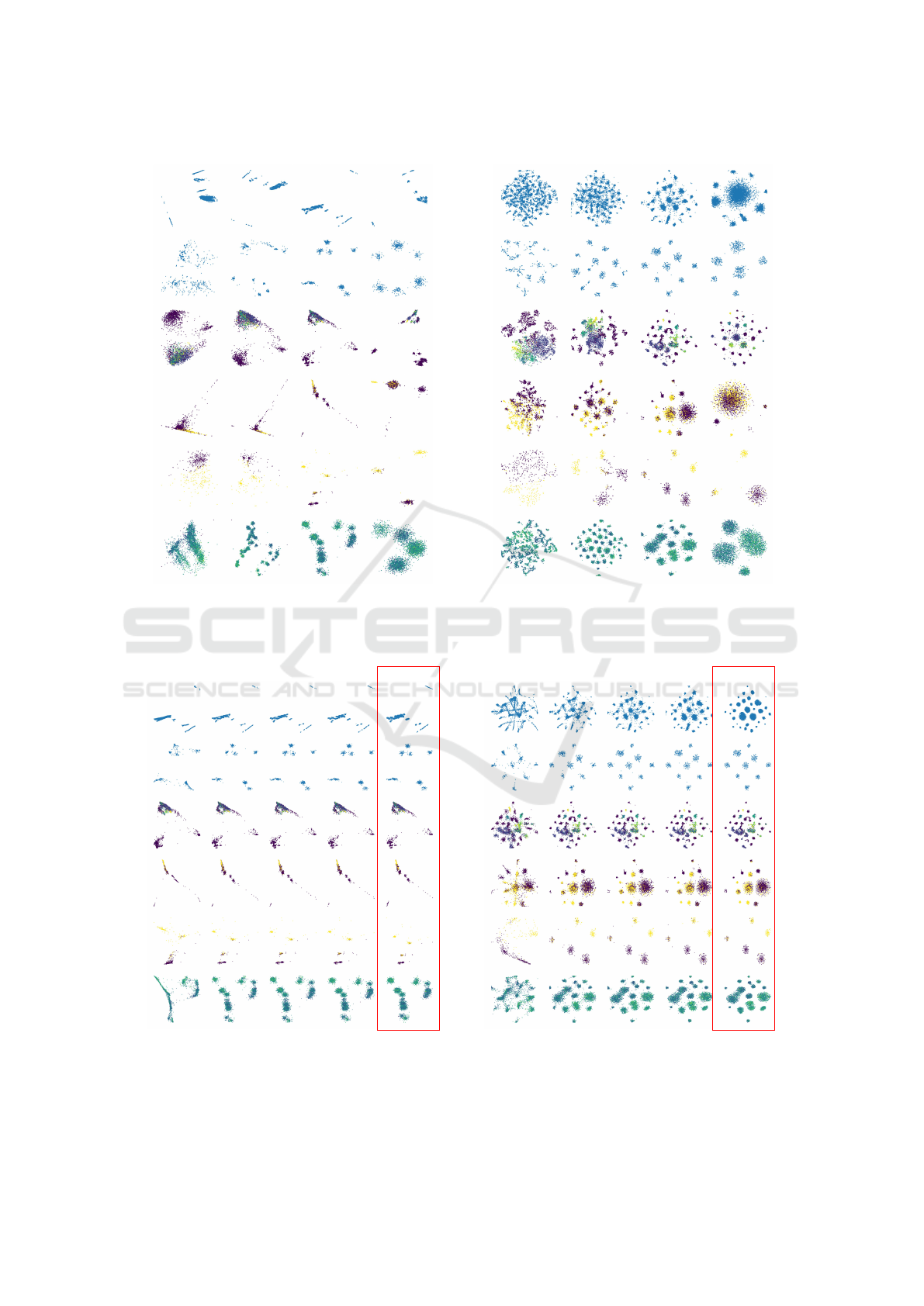
0.01 0.05 0.1 0.2

Wine Wisconsin Spambase Reuters Concrete Air Quality

(a) LMDS.

0.01 0.05 0.1 0.2

Wine Wisconsin Spambase Reuters Concrete Air Quality

(b) t-SNE.

Figure 3: Learning rate effect: SDR-NNP learned from LMDS (a) and t-SNE (b) for varying learning rates α (columns) and

datasets (rows). Fixed SDR-NNP parameters are T = 10 iterations, E = 1000 epochs, medium network size.

Early Stopping 300 ep 1000 ep 3000 ep Training

Wine Wisconsin Spambase Reuters Concrete Air Quality

(a) LMDS.

Early Stopping 300 ep 1000 ep 3000 ep Training

Wine Wisconsin Spambase Reuters Concrete Air Quality

(b) t-SNE.

Figure 4: SDR-NNP learned from LMDS (a) and t-SNE (b) for varying training epochs E (columns) and datasets (rows).

Fixed SDR-NNP parameters are T = 10, α = 0.1, medium network size. Red column shows the training projections.

SDR-NNP: Sharpened Dimensionality Reduction with Neural Networks

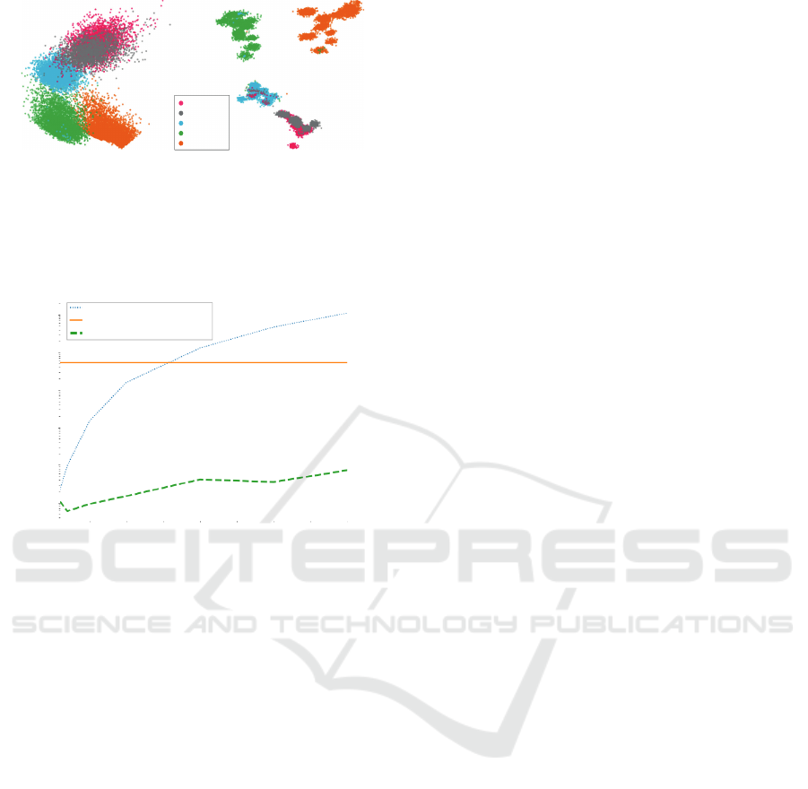
(a) (b)

Running

Dancing

Walking

Standing

Sitting

Figure 5: (a) LMDS and (b) SDR with LMDS baseline

(α = 0.2, T = 10, k

= 100) applied to Human Activity Data

(N=24075, n=60), which was originally tested by Kim et

al. (Kim et al., 2021). Points are colored by their labels on

different human activities (sit, stand, walk, run, and dance).

These results demonstrate the advantage of using sharpen-

ing for data that are known to have cluster structures.

number of samples (x1000)

20 25 30 35

-1

time (seconds, log scale)

SDR

SDR-NNP (train 10K + inference)

SDR-NNP (inference only)

Figure 6: Performance of SDR vs SDR-NNP on the

GALAH dataset (time in log scale), 1K to 40K samples.

SDR-NNP trained with 10K samples for 1000 epochs. See

also Tab. 6.

sion of the training projection (Fig. 4a,b rightmost

columns). This is explained by the fact that SDR-

NNP needs to learn both the data sharpening and the

projection P, which needs more effort than learning

just the projection, as NNP did. If we use more train-

ing epochs, Fig. 4 shows that SDR-NNP can repro-

duce the training projection very faithfully. SDR-

NNP produces good results with as little as E = 300

epochs, except for the Air Quality dataset, where

E = 3000 epochs was needed for best results. On av-

erage, E = 1000 epochs produced visually good re-

sults for all datasets and other parameter settings, so

we choose this as a preset value for E.

The projections in Figs. 2–4 deserve some com-

ments. As visible there, varying the T and α pa-

rameters can create artiﬁcial oversegmentation – the

appearance of many small clusters in the projection,

which is an artiﬁcial cluster separation (CS), see e.g.

Fig. 3b, Reuters, α ≥ 0.1. This effect is strongest,

and undesirable, for baseline projections which al-

ready do have a good CS, such as t-SNE. In contrast,

for projections with a low CS, such as LMDS, artiﬁ-

cial oversegmentation is far less present. Like SDR,

SDR-NNP is best used when combined with baseline

DR methods with a low CS capability.

Separately, as outlined in (Kim et al., 2021), SDR

performs best, and is meant to be used for, datasets

that are known to have cluster structures since sharp-

ening, by construction, will enhance these struc-

tures (Comaniciu and Meer, 2002). SDR-NNP inher-

its these aspects from SDR and, as Fig. 4 shows, can

reproduce SDR highly accurately, and is much faster

(see next Sec. 4.2).

To clarify the above, Fig. 5 shows an example

where SDR shows far better CS compared with a

baseline DR method (LMDS) when applied to real-

world human activity data, which is known to have

distinct and well separated features among different

human motions (sit, stand, walk, run, and dance) (El

Helou, 2020). Even though the points are known to be

well-separated, LMDS produces a relatively low CS

(clusters overlap in Fig. 5a). In contrast, SDR pro-

duces a much higher CS (Fig. 5b), in line with the

ground truth. A second example illustrating the same

point is discussed in detail in Sec. 4.3.

4.2 Computational Scalability

We measured scalability by comparing the execution

time of the original SDR method with SDR-NNP us-

ing samples from the GALAH dataset (described next

in Sec. 4.3) with increasing sizes, namely, 1K, 2K,

5K, 10K, 20K, 30K, and 40K samples. Using more

samples was not practical since SDR already took

over three hours at 40K samples. Figure 6 and Ta-

ble 5 show these ﬁgures. For |D

| = 10K training

samples and E = 1000 epochs, SDR-NNP takes con-

siderable time to train, i.e., 372.818 seconds (Fig. 6,

orange line). Still, this is already faster than SDR

for 15K samples. In inference mode (after training),

SDR-NNP is orders of magnitude faster than SDR,

taking less than one second to project 40K samples

(Fig. 6, green curve). SDR takes over three hours for

the same data size (Fig. 6, blue curve).

4.3 Case Study: Astronomical Datasets

We applied SDR-NNP to a practical use-case using

real-world astronomical data. We use here the same

subset of 10K samples from the GALactic Archaeol-

ogy with HERMES survey (GALAH DR2) (Buder et

al., 2018) as in Kim et al. to show that our method can

create similar projections to their SDR method. The

original GALAH DR2 dataset consists of various stel-

lar abundance attributes of 342682 stars. Data clean-

ing followed (Kim et al., 2021): ﬁrst, cross-match

the star ID of GALAH DR2 with Gaia data release

2 (Gaia DR2) to gain additional information on the

IVAPP 2022 - 13th International Conference on Information Visualization Theory and Applications

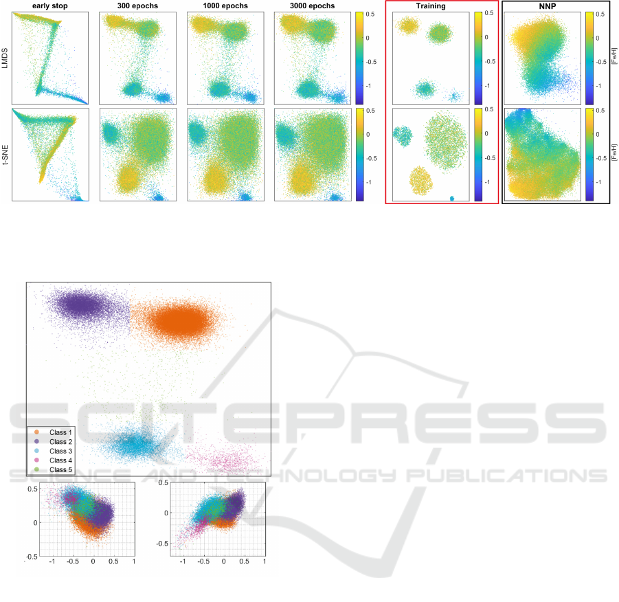
Figure 7: SDR-NNP of 66K samples learned from LMDS (top) and t-SNE (bottom) for different numbers of training epochs

E (four leftmost columns). SDR-NNP parameters are T = 10 iterations, α = 0.18, and medium network size. Red column:

training projection (10K samples). Rightmost column: NNP trained with LMDS and t-SNE instead of SDR applied to the

same test data.

[Mg/Fe]

[Fe/H]

[Cu/Fe]

[Fe/H]

b) c)

Figure 8: Analysis of GALAH DR2 with SDR-NNP

learned from LMDS. (a) Labeling of clusters (classes 1–4)

and outliers (class 5). (b) Tinsley diagram and (c) copper

abundance of stars vs their iron abundance. Astronomers

can infer from (b,c) that class 1 is mostly thin disk stars,

class 2 is mostly metal-rich thick disk stars, classes 5 and

3 are normal thick disk stars, and class 4 is the Gaia Ence-

ladus (GES) in the Milky Way.

stellar kinematics (i.e., 6D phase-space coordinates–

x, y, z, u, v, and w) (Buder et al., 2018; Gaia Collab-

oration, 2016; Gaia Collaboration, 2018); next, ex-

clude stars with implausible values (exceeding 25K

parsec in x, y, and z attributes), having unreliable stel-

lar abundances, or have missing values in any dimen-

sion. From the remaining 76270 samples after pre-

processing, we took the same subset D of 10K stars as

in (Kim et al., 2021), where stars were randomly se-

lected, and compute SDR and the training projection

with the same α = 0.18 (see Sec. 3.1). We trained

SDR-NNP on these 10K stars and used the trained

network to project the remaining 66270 samples.

Figure 7 shows SDR-NNP applied to the 66K test

data with LMDS and t-SNE as baseline DR methods.

Points are colored based on the value of the attribute

[Fe/H], which is of interest to domain experts to ex-

plain possible data clusters. The ﬁrst four columns

show the SDR-NNP results for varying training epoch

counts E. The red column shows the training projec-

tion P(D

) of 10K samples. We see that the structure

of the training projection (four clusters) is well re-

ﬂected by the SDR-NNP results from E = 300 epochs

onwards. The test projections are more fuzzy, but

this is expected, as these contain 66K unseen sam-

ples which, albeit drawn from the same dataset, can-

not perfectly match the four clusters determined by

the 10K training samples. The rightmost column in

Fig. 7 shows the result of the ‘raw’ NNP method,

i.e., trained to imitate LMDS, and t-SNE, without the

sharpening step of SDR, respectively. These results

show clearly far less cluster separation (CS) than ei-

ther the SDR-NNP training projection (red column)

or the inferred SDR-NNP projections (leftmost four

columns). This demonstrates the added value of the

sharpening step: without it, NNP, albeit fast and

OOS-capable, cannot produce useful projections. Ta-

ble 6 in the Appendix shows quality metrics corre-

sponding to the images in Fig. 7 which support the

above observations.

The fact that SDR-NNP shows a good cluster sep-

aration allows astronomers to easily label clusters and

perform further analysis to infer the physical meaning

of stars. To demonstrate this, we manually labeled the

clusters from the SDR-NNP plot learned from LMDS

SDR-NNP: Sharpened Dimensionality Reduction with Neural Networks

to reproduce the same analyses made by Kim et al.

(Fig. 10 in (Kim et al., 2021)) to understand the ori-

gin and location of the stars in each cluster. Figure 8a

shows the manually labeled clusters by one of the au-

thors (astronomy expert). Stars from class 5 are sepa-

rately labeled as outliers. Figures 8b,c are the Tinsley

diagram (Tinsley, 1980) and the copper abundance of

the stars – a tracer of supernovae type 1a – as a func-

tion of their iron abundance, respectively. From these

plots, astronomers are able to identify class-1 stars as

thin-disk stars, class-2 stars as metal-rich thick disk

stars, class-3 and class-5 (outlier) stars as the normal

thick disk stars, and class-4 stars as Gaia Enceladus

(GES) – a group of stars that originated from a galaxy

that merged with the Milky Way several billions years

ago. Importantly, the original SDR method was not

able to perform this analysis and identify class-4 stars

since it could not be applied to the entire dataset due

to its prohibitively low speed.

4.4 Implementation Details

All experiments were run on a dual 16-core Intel

Xeon Silver 4216 at 2.1 GHz with 256 GB RAM

and an NVidia GeForce GTX 1080 Ti GPU with 11

GB VRAM. SDR was implemented in C++ using

Eigen (Guennebaud et al., 2010) for matrix computa-

tions, Nanoﬂann (Blanco and Rai, 2014) for nearest-

neighbor search, and the implementations of t-SNE

and Landmark MDS from Tapkee (Lisitsyn et al.,

2013). NNP is implemented using the Keras frame-

work (Chollet and others, 2015). The SDR-NNP

code, datasets, and all results discussed above are

publicly available at (Kim et al., 2021a).

5 DISCUSSION

We discuss how SDR-NNP performs with respect to

the criteria laid out in Sec. 1.

Quality (C1): SDR-NNP is able to create projections

which are very similar visually, but also in terms of

quality metrics, to those created by SDR. Importantly,

the strong separation of similar-valued samples, the

key property that SDR promoted, is retained by SDR-

NNP. Combined with properties C2–C4 (which SDR

does not have), this makes SDR-NNP superior to

SDR. Compared to NNP used on the unsharpened

data (Fig. 7), SDR-NNP shows signiﬁcantly better

cluster separation, which makes it superior to NNP.

Scalability (C2): SDR-NNP is faster than SDR alone

from roughly 15K samples onwards, even when con-

sidering training time. In inference mode (after train-

ing), SDR-NNP is several orders of magnitude faster

than SDR, being able to project tens of thousands of

observations in under a second on a high-end PC. Im-

portantly, SDR-NNP’s speed is linear in the number

of dimensions and samples (a property inherited from

the NNP architecture), and can handle samples in a

streaming fashion, one at a time, i.e, does not need

to hold the entire high-dimensional dataset in mem-

ory. This makes SDR-NNP scalable to large datasets

of millions of samples.

Ease of Use (C3): Once trained, SDR-NNP is

parameter-free. The inﬂuence of its hyperparame-

ters T (sharpening iterations), E (number of training

epochs), and α (learning rate) is detailed in Sec. 4.1.

The preset T = 10,E = 1000,α ' 0.2 was shown

to give good results for the entire range of tested

datasets.

Genericity (C4): SDR-NNP is agnostic to the nature

and dimensionality of the input data, being able to

project any dataset having quantitative variables. Ta-

bles 6, 7, and 8 in the Appendix show that SDR-NNP

achieves high quality on datasets of different nature

and coming from a wide range of application domains

(air sensors, civil engineering, text mining, imaging,

and chemistry).

Stability and Out-of-Sample Support (C5): SDR-

NNP inherits the stability and OOS support of NNP,

making it possible to train on a small subset of a

given dataset and then stably project the remaining

data drawn from the same distribution.

Limitations: While inheriting the abovementioned

desirable properties from NNP, SDR-NNP also inher-

its some of its limitations. Its OOS support cannot ex-

tend to datasets of a completely different nature than

those it was trained on – arguably, a limitation that

most machine learning methods have. Also, SDR-

NNP is only as good as the baseline projection P that

was used in the SDR phase. Using a poor quality pro-

jection leads to SDR-NNP learning, and reproducing,

that behavior. Separately, SDR-NNP learns to imi-

tate the sharpening behavior of SDR. While this is of

added value in identifying data structure in terms of

visual structure, as shown by the results in Sec. 4, ap-

plying SDR-NNP on a dataset with little or no clus-

ter structure can create artiﬁcial visual oversegmen-

tation in the projection (see Sec. 4.1). The recom-

mended parameter values to prevent oversegmenta-

tion using SDR are discussed further in Sec. 6.5 in

(Kim et al., 2021). Specifying the right amount of

sharpening is dataset- and problem-dependent, thus

considered as future work.

IVAPP 2022 - 13th International Conference on Information Visualization Theory and Applications

6 CONCLUSION

We have presented SDR-NNP, a new method for com-

puting projections of high-dimensional datasets for

visual exploration purposes. Our method joins sev-

eral desirable, and complementary, characteristics of

two earlier projection methods, namely NNP (speed,

ease of use, out-of-sample support, ability to imitate

a wide range of existing projection techniques with

a high quality) and SDR (ability to segregate projec-

tions of complex datasets into visually separated clus-

ters of similar observations). In particular, SDR-NNP

removes the main obstacle for practical usage of SDR,

namely, its prohibitive computational time. We have

demonstrated SDR-NNP on a range of datasets com-

ing from different application domains. In particu-

lar, we showed how SDR-NNP can bring added value

in the exploration of a large and recent astronomical

dataset leading to ﬁndings which were not achievable

by SDR or NNP alone.

Future work can target several directions. As

SDR-NNP showed that it is possible to learn sharp-

ening methods for high-dimensional data, it is inter-

esting to apply it to other domains beyond projection

where such methods are used, e.g., image segmenta-

tion, graph bundling, or data clustering and simpli-

ﬁcation. For the projection use-case, reﬁning SDR-

NNP’s network architecture to accelerate its training

is of high practical interest. Finally, deploying SDR-

NNP as a daily tool for astronomers to analyze their

million-sample datasets is a goal we want to pursue in

the short term.

ACKNOWLEDGMENTS

This work is supported by the DSSC Doctoral Train-

ing Programme co-funded by the Marie Sklodowska-

Curie COFUND project (DSSC 754315), and

FAPESP grant 2020/13275-1, Brazil. The GALAH

survey is based on observations made at the

Australian Astronomical Observatory, under pro-

grammes A/2013B/13, A/2014A/25, A/2015A/19,

A/2017A/18. We acknowledge the traditional

owners of the land on which the AAT stands, the

Gamilaraay people, and pay our respects to elders

past and present. This work has made use of data

from the European Space Agency (ESA) mission

Gaia (https://www.cosmos.esa.int/gaia), processed

by the Gaia Data Processing and Analysis Con-

sortium (DPAC, https://www.cosmos.esa.int/web/

gaia/dpac/consortium). Funding for the DPAC has

been provided by national institutions, in particu-

lar the institutions participating in the Gaia Multilat-

eral Agreement.

REFERENCES

Agarap, A. F. (2018). Deep learning using rectiﬁed linear

units (ReLU). arXiv:1803.08375 [cs.NE].

Becker, M., Lippel, J., Stuhlsatz, A., and Zielke, T. (2020).

Robust dimensionality reduction for data visualiza-

tion with deep neural networks. Graphical Models,

108:101060.

Becker, R., Cleveland, W., and Shyu, M. (1996). The visual

design and control of trellis display. J Comp Graph

Stat, 5(2):123–155.

Behrisch, M., Blumenschein, M., Kim, N. W., Shao, L., El-

Assady, M., Fuchs, J., Seebacher, D., Diehl, A., Bran-

des, U., Pﬁster, H., Schreck, T., Weiskopf, D., and

Keim, D. A. (2018). Quality metrics for information

visualization. Comp Graph Forum, 37(3):625–662.

Berkhin, P. (2006). A survey of clustering data mining tech-

niques. In Grouping Multidimensional Data, pages

25–71. Springer.

Blanco, J. L. and Rai, P. K. (2014). nanoﬂann: a C++

header-only fork of FLANN, a library for nearest

neighbor (NN) with kd-trees. https://github.com/

jlblancoc/nanoﬂann.

Buder et al., S. (2018). The GALAH Survey: Second data

release. Mon R R Astron Soc, 478.

Chan, D., Rao, R., Huang, F., and Canny, J. (2018). T-SNE-

CUDA: GPU-accelerated t-SNE and its applications

to modern data. In Proc. SBAC-PAD, pages 330–338.

Cheng, Y. (1995). Mean shift, mode seeking, and clustering.

IEEE TPAMI, 17(8):790–799.

Chollet, F. and others (2015). Keras. https://keras.io.

Comaniciu, D. and Meer, P. (2002). Mean shift: A robust

approach toward feature space analysis. IEEE TPAMI,

24(5):603–619.

Cortez, P., Cerdeira, A., Almeida, F., Matos, T., and Reis,

J. (2009). Modeling wine preferences by data mining

from physicochemical properties. Decis Support Sys,

47(4):547–553.

Cunningham, J. and Ghahramani, Z. (2015). Linear dimen-

sionality reduction: Survey, insights, and generaliza-

tions. JMLR, 16:2859–2900.

De Silva, V. and Tenenbaum, J. B. (2004). Sparse multidi-

mensional scaling using landmark points. Technical

report, Stanford University.

Donoho, D. L. and Grimes, C. (2003). Hessian eigen-

maps: Locally linear embedding techniques for high-

dimensional data. PNAS, 100(10):5591–5596.

El Helou, A. (2020). Sensor HAR recognition app.

www.mathworks.com/matlabcentral/ﬁleexchange/

54138-sensor-har-recognition-app.

Engel, D., Hattenberger, L., and Hamann, B. (2012). A

survey of dimension reduction methods for high-

dimensional data analysis and visualization. In Proc.

IRTG Workshop, volume 27, pages 135–149. Schloss

Dagstuhl.

SDR-NNP: Sharpened Dimensionality Reduction with Neural Networks

Epanechnikov, V. (1969). Non-parametric estimation of a

multivariate probability density. Theor Probab Appl+,

14.

Espadoto, M., Hirata, N., and Telea, A. (2020). Deep

learning multidimensional projections. Inform Visual,

9(3):247–269.

Espadoto, M., Hirata, N., and Telea, A. (2021). Self-

supervised dimensionality reduction with neural net-

works and pseudo-labeling. In Proc. IVAPP.

Espadoto, M., Martins, R., Kerren, A., Hirata, N., and

Telea, A. (2019). Toward a quantitative survey

of dimension reduction techniques. IEEE TVCG,

27(3):2153–2173.

Fisher, R. A. (1936). The use of multiple measurements in

taxonomic problems. Annals of eugenics, 7(2):179–

188.

Fukunaga, K. and Hostetler, L. (1975). The estimation of

the gradient of a density function, with applications in

pattern recognition. IEEE Trans Inf Theor, 21(1):32–

40.

Gaia Collaboration (2016). The Gaia mission. Astronomy

& Astrophysics, 595, A1.

Gaia Collaboration (2018). Gaia Data Release 2-Summary

of the contents and survey properties. Astronomy &

Astrophysics, 616, A1.

Guennebaud, G., Jacob, B., et al. (2010). Eigen v3.

http://eigen.tuxfamily.org.

He, K., Zhang, X., Ren, S., and Sun, J. (2015). Delving

deep into rectiﬁers: Surpassing human-level perfor-

mance on ImageNet classiﬁcation. In Proc. ICCV,

pages 1026–1034.

Hinton, G. E. and Salakhutdinov, R. R. (2006). Reducing

the dimensionality of data with neural networks. Sci-

ence, 313(5786):504–507. Publisher: AAAS.

Hoffman, P. and Grinstein, G. (2002). A survey of visual-

izations for high-dimensional data mining. In Infor-

mation Visualization in Data Mining and Knowledge

Discovery, pages 47–82.

Hopkins, M., Reeber, E., Forman, G., and Suermondt, J.

(1999). Spambase dataset. Hewlett-Packard Labs.

Hurter, C., Ersoy, O., and Telea, A. (2012). Graph bundling

by kernel density estimation. Comp Graph Forum,

31(3):865–874.

Inselberg, A. and Dimsdale, B. (1990). Parallel coordinates:

A tool for visualizing multi-dimensional geometry. In

Proc. IEEE Visualization, pages 361–378.

Joia, P., Coimbra, D., Cuminato, J. A., Paulovich, F. V., and

Nonato, L. G. (2011). Local afﬁne multidimensional

projection. IEEE TVCG, 17(12):2563–2571.

Jolliffe, I. T. (1986). Principal component analysis and fac-

tor analysis. In Principal Component Analysis, pages

115–128. Springer.

Kim, Y., Telea, A., Trager, S., and Roerdink, J. B.

T. M. (2021). Visual cluster separation using

high-dimensional sharpened dimensionality reduc-

tion. arXiv:2110.00317 [cs.CV].

Kim, Y., Espadoto, M., Trager, S. C., Roerdink, J. B. T. M.,

and Telea, A. C. (2021a). SDR-NNP implementation

and results. https://github.com/youngjookim/sdr-nnp.

Kingma, D. P. and Ba, J. (2014). Adam: A method for

stochastic optimization. arXiv:1412.6980.

Kingma, D. P. and Welling, M. (2013). Auto-encoding

variational bayes. CoRR, abs/1312.6114. eprint:

1312.6114.

Kohonen, T. (1997). Self-organizing Maps. Springer.

LeCun, Y. and Cortes, C. (2010). MNIST handwritten digits

dataset. http://yann.lecun.com/exdb/mnist.

Lisitsyn, S., Widmer, C., and Garcia, F. J. I. (2013). Tap-

kee: An efﬁcient dimension reduction library. JMLR,

14:2355–2359.

Liu, S., Maljovec, D., Wang, B., Bremer, P.-T., and

Pascucci, V. (2015). Visualizing high-dimensional

data: Advances in the past decade. IEEE TVCG,

23(3):1249–1268.

Maaten, L. v. d. (2014). Accelerating t-SNE using tree-

based algorithms. JMLR, 15:3221–3245.

Maaten, L. v. d. and Hinton, G. (2008). Visualizing data

using t-SNE. JMLR, 9:2579–2605.

Maaten, L. v. d. and Postma, E. (2009). Dimensionality

reduction: A comparative review. Technical report,

Tilburg Univ.

Martins, R. M., Minghim, R., Telea, A. C., and others

(2015). Explaining neighborhood preservation for

multidimensional projections. In Proc. CGVC, pages

7–14.

McInnes, L. and Healy, J. (2018). UMAP: Uniform man-

ifold approximation and projection for dimension re-

duction. arXiv:1802.03426v1 [stat.ML].

Nonato, L. and Aupetit, M. (2018). Multidimensional

projection for visual analytics: Linking techniques

with distortions, tasks, and layout enrichment. IEEE

TVCG.

Paulovich, F. V. and Minghim, R. (2006). Text map ex-

plorer: a tool to create and explore document maps.

In Proc. Information Visualisation, pages 245–251.

IEEE.

Paulovich, F. V., Nonato, L. G., Minghim, R., and Lev-

kowitz, H. (2008). Least square projection: A fast

high-precision multidimensional projection technique

and its application to document mapping. IEEE

TVCG, 14(3):564–575.

Pezzotti, N., H

ollt, T., Lelieveldt, B., Eisemann, E., and

Vilanova, A. (2016). Hierarchical stochastic neighbor

embedding. Comp Graph Forum, 35(3):21–30.

Pezzotti, N., Lelieveldt, B., Maaten, L. v. d., H

ollt, T., Eise-

mann, E., and Vilanova, A. (2017). Approximated and

user steerable t-SNE for progressive visual analytics.

IEEE TVCG, 23:1739–1752.

Pezzotti, N., Thijssen, J., Mordvintsev, A., Hollt, T., Lew,

B. v., Lelieveldt, B., Eisemann, E., and Vilanova, A.

(2020). GPGPU linear complexity t-SNE optimiza-

tion. IEEE TVCG, 26(1):1172–1181.

Rao, R. and Card, S. K. (1994). The table lens: Merging

graphical and symbolic representations in an interac-

tive focus+context visualization for tabular informa-

tion. In Proc. ACM SIGCHI, pages 318–322.

Rauber, P. E., Falc

ao, A. X., and Telea, A. C. (2017). Pro-

jections as visual aids for classiﬁcation system design.

Inform Visual, 17(4):282–305.

Roweis, S. T. and Saul, L. L. K. (2000). Nonlinear dimen-

sionality reduction by locally linear embedding. Sci-

ence, 290(5500):2323–2326.

IVAPP 2022 - 13th International Conference on Information Visualization Theory and Applications

Salton, G. and McGill, M. J. (1986). Introduction to modern

information retrieval. McGraw-Hill.

Sorzano, C., Vargas, J., and Pascual-Montano, A. (2014).

A survey of dimensionality reduction techniques.

arXiv:1403.2877 [stat.ML].

Street, N., Wolberg, W., and Mangasarian, O. (1993). Nu-

clear feature extraction for breast tumor diagnosis. In

Biomedical image processing and biomedical visual-

ization, volume 1905, pages 861–870.

Tenenbaum, J. B., Silva, V. D., and Langford, J. C. (2000).

A global geometric framework for nonlinear dimen-

sionality reduction. Science, 290(5500):2319–2323.

Thoma, M. (2017). The Reuters dataset. https://

martin-thoma.com/nlp-reuters.

Tinsley, B. (1980). Evolution of the stars and gas in galax-

ies. Fundamentals of Cosmic Physics, 5:287–388.

Torgerson, W. (1958). Theory and Methods of Scaling. Wi-

ley.

Venna, J. and Kaski, S. (2006). Visualizing gene interaction

graphs with local multidimensional scaling. In Proc.

ESANN, pages 557–562.

Vito, S. D., Massera, E., Piga, M., Martinotto, L., and Fran-

cia, G. D. (2008). On ﬁeld calibration of an elec-

tronic nose for benzene estimation in an urban pol-

lution monitoring scenario. Sensors and Actuators

B: Chemical, 129(2):750–757. https://archive.ics.uci.

edu/ml/datasets/Air+Quality.

Wattenberg, M. (2016). How to use t-SNE effectively. https:

//distill.pub/2016/misread-tsne.

Xie, H., Li, J., and Xue, H. (2017). A survey of dimen-

sionality reduction techniques based on random pro-

jection. arXiv:1706.04371 [cs.LG].

Xu, R. and Wunsch, D. (2005). Survey of clustering al-

gorithms. IEEE Transactions on Neural Networks,

16(3):645–678.

Yates, A., Webb, A., Sharpnack, M., Chamberlin, H.,

Huang, K., and Machiraju, R. (2014). Visualizing

multidimensional data with glyph SPLOMs. Comp

Graph Forum, 33(3):301–310.

Yeh, I.-C. (1998). Modeling of strength of high-

performance concrete using artiﬁcial neural networks.

Cement and Concrete Research, 28(12):1797–1808.

Zhang, Z. and Wang, J. (2007). MLLE: Modiﬁed locally

linear embedding using multiple weights. In Proc.

NIPS, pages 1593–1600.

Zhang, Z. and Zha, H. (2004). Principal manifolds and

nonlinear dimensionality reduction via tangent space

alignment. SIAM J Sci Comput, 26(1):313–338.

SDR-NNP: Sharpened Dimensionality Reduction with Neural Networks

APPENDIX

We next present tables containing full measurements

for the experiments described in Section 4.

Table 6: Metrics for SDR-NNP learned from LMDS, PCA, and t-SNE on the GALAH dataset for train and test samples for

varying number of training epochs E (‘early’ indicates the early-stopping heuristic).

LMDS PCA t-SNE

Mode Epochs T C R T C R T C R

Train

early 0.802 0.877 0.676 0.787 0.853 0.668 0.789 0.870 0.638

300 0.703 0.790 0.629 0.697 0.778 0.617 0.694 0.770 0.496

1000 0.695 0.772 0.615 0.693 0.762 0.607 0.692 0.748 0.481

3000 0.692 0.756 0.600 0.693 0.756 0.601 0.691 0.734 0.447

Test

early 0.775 0.862 0.601 0.754 0.828 0.592 0.756 0.853 0.574

300 0.667 0.768 0.558 0.660 0.759 0.544 0.652 0.755 0.470

1000 0.661 0.749 0.547 0.658 0.746 0.539 0.642 0.734 0.449

3000 0.657 0.737 0.534 0.655 0.739 0.539 0.641 0.720 0.416

Table 7: Metrics for SDR-NNP learned from LMDS, PCA, and t-SNE for different numbers of iterations T and different

datasets. SDR-NNP parameters used: α = 0.1, E = 1000, medium network size. NH values not available for the Air Quality

and Concrete datasets since these are not labeled.

LMDS PCA t-SNE

Dataset SDR iterations T C R NH T C R NH T C R NH

Air Quality

0 0.941 0.992 0.970 0.940 0.992 0.966 0.996 0.996 0.654

4 0.962 0.979 0.963 0.956 0.979 0.963 0.951 0.939 0.396

8 0.954 0.970 0.952 0.942 0.970 0.948 0.945 0.938 0.313

12 0.949 0.970 0.952 0.945 0.970 0.936 0.942 0.942 0.365

16 0.950 0.968 0.943 0.948 0.967 0.930 0.940 0.933 0.317

20 0.954 0.968 0.939 0.949 0.967 0.917 0.943 0.939 0.334

Concrete

0 0.940 0.979 0.744 0.934 0.977 0.736 0.996 0.992 0.479

4 0.938 0.958 0.631 0.934 0.957 0.627 0.952 0.929 0.145

8 0.912 0.944 0.560 0.906 0.943 0.564 0.927 0.918 0.140

12 0.895 0.941 0.556 0.865 0.932 0.558 0.912 0.913 0.167

16 0.884 0.938 0.554 0.872 0.932 0.555 0.904 0.914 0.118

20 0.876 0.935 0.560 0.874 0.934 0.569 0.890 0.910 0.109

Reuters

0 0.817 0.895 0.755 0.724 0.817 0.888 0.754 0.727 0.956 0.960 0.609 0.856

4 0.835 0.913 0.752 0.747 0.833 0.901 0.745 0.743 0.957 0.951 0.405 0.855

8 0.858 0.915 0.713 0.775 0.854 0.906 0.706 0.765 0.950 0.910 0.258 0.845

12 0.883 0.909 0.693 0.803 0.883 0.904 0.687 0.802 0.915 0.855 0.078 0.820

16 0.884 0.910 0.691 0.810 0.882 0.907 0.689 0.804 0.893 0.849 0.102 0.813

20 0.882 0.907 0.691 0.800 0.883 0.907 0.691 0.810 0.893 0.852 0.113 0.820

Spambase

0 0.740 0.909 0.529 0.852 0.747 0.912 0.513 0.849 0.954 0.958 0.408 0.914

4 0.737 0.881 0.463 0.843 0.743 0.877 0.471 0.841 0.873 0.899 0.294 0.882

8 0.723 0.855 0.403 0.838 0.712 0.848 0.383 0.834 0.793 0.845 0.312 0.866

12 0.711 0.845 0.379 0.829 0.704 0.838 0.348 0.830 0.754 0.841 0.324 0.850

16 0.701 0.837 0.370 0.828 0.701 0.837 0.322 0.830 0.744 0.834 0.332 0.845

20 0.710 0.840 0.351 0.833 0.709 0.838 0.311 0.836 0.739 0.828 0.283 0.848

Wisconsin

0 0.895 0.959 0.926 0.941 0.896 0.959 0.928 0.943 0.950 0.939 0.679 0.976

4 0.892 0.915 0.901 0.953 0.888 0.915 0.903 0.958 0.897 0.878 0.557 0.957

8 0.804 0.857 0.785 0.925 0.805 0.856 0.785 0.925 0.814 0.816 0.256 0.925

12 0.790 0.849 0.735 0.930 0.787 0.848 0.736 0.930 0.794 0.805 0.393 0.932

16 0.780 0.847 0.721 0.916 0.780 0.844 0.718 0.922 0.779 0.820 0.432 0.913

20 0.775 0.842 0.707 0.922 0.776 0.841 0.705 0.920 0.778 0.829 0.457 0.921

Wine

0 0.864 0.973 0.839 0.667 0.869 0.972 0.806 0.678 0.986 0.976 0.656 0.702

4 0.867 0.932 0.709 0.669 0.864 0.930 0.686 0.665 0.911 0.894 0.341 0.673

8 0.843 0.916 0.676 0.661 0.843 0.917 0.683 0.661 0.869 0.876 0.283 0.665

12 0.840 0.904 0.646 0.665 0.841 0.905 0.653 0.668 0.846 0.864 0.289 0.668

16 0.845 0.901 0.625 0.664 0.843 0.903 0.635 0.663 0.845 0.865 0.321 0.664

20 0.842 0.899 0.579 0.659 0.846 0.898 0.593 0.664 0.845 0.868 0.292 0.666

Table 8: Metrics for SDR-NNP learned from LMDS, PCA, and t-SNE for different learning rates α. SDR-NNP parameters:

T = 10 iterations, E = 1000 epochs, medium network. NH values not available for the Air Quality and Concrete datasets

since these are not labeled.

LMDS PCA t-SNE

Dataset Learning Rate T C R NH T C R NH T C R NH

Air Quality

0.01 0.971 0.990 0.969 0.968 0.990 0.964 0.958 0.926 0.052

0.05 0.976 0.983 0.963 0.973 0.984 0.964 0.938 0.911 0.175

0.1 0.951 0.969 0.948 0.940 0.969 0.941 0.943 0.939 0.378

0.2 0.866 0.941 0.911 0.862 0.928 0.905 0.824 0.876 0.635

Concrete

0.01 0.959 0.983 0.731 0.950 0.979 0.721 0.994 0.988 0.486

0.05 0.932 0.957 0.601 0.929 0.953 0.601 0.947 0.929 0.219

0.1 0.870 0.933 0.578 0.889 0.935 0.583 0.913 0.918 0.057

0.2 0.858 0.920 0.540 0.859 0.921 0.542 0.857 0.900 0.223

Reuters

0.01 0.822 0.900 0.758 0.729 0.821 0.892 0.755 0.730 0.956 0.960 0.608 0.853

0.05 0.839 0.913 0.737 0.745 0.838 0.903 0.735 0.745 0.955 0.949 0.386 0.849

0.1 0.870 0.910 0.698 0.783 0.871 0.905 0.693 0.790 0.936 0.885 0.159 0.829

0.2 0.866 0.902 0.700 0.784 0.867 0.903 0.693 0.785 0.890 0.848 0.096 0.815

Spambase

0.01 0.755 0.911 0.527 0.860 0.756 0.915 0.523 0.852 0.958 0.942 0.383 0.905

0.05 0.775 0.893 0.415 0.840 0.787 0.894 0.426 0.858 0.851 0.874 0.261 0.874

0.1 0.712 0.843 0.380 0.832 0.704 0.839 0.367 0.828 0.769 0.848 0.341 0.863

0.2 0.604 0.667 0.265 0.760 0.606 0.671 0.263 0.764 0.635 0.676 0.317 0.802

Wisconsin

0.01 0.900 0.960 0.932 0.947 0.898 0.960 0.932 0.949 0.955 0.941 0.635 0.966

0.05 0.868 0.885 0.869 0.946 0.874 0.890 0.870 0.941 0.876 0.861 0.597 0.948

0.1 0.803 0.856 0.757 0.928 0.800 0.851 0.753 0.929 0.802 0.841 0.494 0.927

0.2 0.717 0.764 0.693 0.905 0.718 0.758 0.684 0.918 0.725 0.749 0.596 0.909

Wine

0.01 0.895 0.972 0.811 0.674 0.898 0.971 0.783 0.681 0.983 0.951 0.448 0.696

0.05 0.914 0.944 0.734 0.671 0.920 0.945 0.714 0.670 0.927 0.862 0.135 0.670

0.1 0.837 0.913 0.672 0.658 0.848 0.913 0.672 0.664 0.864 0.882 0.250 0.661

0.2 0.739 0.821 0.479 0.653 0.742 0.825 0.484 0.644 0.744 0.808 0.404 0.646

IVAPP 2022 - 13th International Conference on Information Visualization Theory and Applications

REFERENCES

Agarap, A. F. (2018). Deep learning using rectified linear