MinMax-CAM: Improving Focus of CAM-based Visualization
Techniques in Multi-label Problems
Lucas David
a
, Helio Pedrini
b
and Zanoni Dias
c
Institute of Computing, University of Campinas, Campinas, Brazil
Keywords:
Computer Vision, Multi-label, Explainable Artificial Intelligence.
Abstract:
The Class Activation Map (CAM) technique (and derivations thereof) has been broadly used in the literature to
inspect the decision process of Convolutional Neural Networks (CNNs) in classification problems. However,
most studies have focused on maximizing the coherence between the visualization map and the position, shape
and sizes of a single object of interest, and little is known about the performance of visualization techniques
in scenarios where multiple objects of different labels coexist. In this work, we conduct a series of tests
that aim to evaluate the efficacy of CAM techniques over distinct multi-label sets. We find that techniques
that were developed with single-label classification in mind (such as Grad-CAM, Grad-CAM++ and Score-
CAM) will often produce diffuse visualization maps in multi-label scenarios, overstepping the boundaries
of their explaining objects onto different labels. We propose a generalization of CAM technique, based on
multi-label activation maximization/minimization to create more accurate activation maps. Finally, we present
a regularization strategy that encourages sparse positive weights in the classifying layer, producing cleaner
activation maps and better multi-label classification scores.
1 INTRODUCTION
Convolutional Neural Networks (CNNs) have become
paramount in the solution of many modern computer
vision problems, such as image classification (Rawat
and Wang, 2017), object detection (Dhillon and
Verma, 2020) and localization, image segmenta-
tion (Minaee et al., 2021) and pose estimation (Wei
et al., 2016). Additionally, CNNs have also shown
great promise when working with unstructured data
from multiple non-imagery domains, such as audio
processing (Pons et al., 2017), text classification (Yao
et al., 2019) and text-to-speech (Tachibana et al.,
2018), with few changes in their original formulation.
In spite of their unquestionable efficacy, their mas-
sive composition of operations degrades overall inter-
pretability, rendering “black box” models. As CNNs
gradually permeate into many real-world systems, im-
pacting different demographics, the necessity for ex-
plaining and accountability becomes urgent.
While the construction of interpretable models is
desirable as a general rule, as it facilitates the iden-
tification of failure modes while hinting strategies to
a
https://orcid.org/0000-0002-8793-7300
b
https://orcid.org/0000-0003-0125-630X
c
https://orcid.org/0000-0003-3333-6822
fix them (Selvaraju et al., 2017), it is also an essential
component in building trust from the general public
towards this technology (Huff et al., 2021).
In this work, we attempt to evaluate and extend
visualization and visual explaining techniques based
on Class Activation Maps (CAMs) onto a multi-label
scenario, in which analysis can be considerably more
challenging (Tarekegn et al., 2021). The main contri-
butions of this work are the following:
1. We propose a thoroughly analysis of popular vi-
sualization techniques in the literature over a dis-
tinct set of multi-label problems, evaluating their
results according to the offered coverage over ob-
jects belonging to the label of interest, as well as
the containment within objects of said label.
2. We propose a modification to CAM-based meth-
ods that combines gradient information from mul-
tiple labels within a single input image. We
demonstrate that our approach presents better
scores and cleaner visualization maps than other
methods over distinct datasets and architectures.
3. We present a regularization strategy that encour-
ages networks to associate each learned label with
a distinct set of patterns, resulting in better sep-
aration of concepts and producing cleaner CAM
visualizations, with better scores.
106
David, L., Pedrini, H. and Dias, Z.
MinMax-CAM: Improving Focus of CAM-based Visualization Techniques in Multi-label Problems.
DOI: 10.5220/0010807800003124
In Proceedings of the 17th International Joint Conference on Computer Vision, Imaging and Computer Graphics Theory and Applications (VISIGRAPP 2022) - Volume 4: VISAPP, pages
106-117
ISBN: 978-989-758-555-5; ISSN: 2184-4321
Copyright
c
 2022 by SCITEPRESS – Science and Technology Publications, Lda. All rights reserved

The remaining of this work is organized as fol-
lows. Section 2 summarizes the explaining methods
currently used in literature. Section 3 describes our
approach in detail, while Section 4 presents the ex-
perimental setup used to evaluate our strategy, the
datasets and network architectures employed. We dis-
cuss our main results in Section 5 and present a reg-
ularization strategy to improve them in Section 6. Fi-
nally, we conclude the paper in Section 7 by remark-
ing our results and proposing future work.
2 RELATED WORK
In the context of computer vision, CNNs are often
inspected with the aid of visual explanation strate-
gies, in which important regions that most contribute
to the answer provided by the aforementioned model
are somehow indicated to the user. Early work in this
vein, namely gradient-based saliency methods (Si-
monyan et al., 2014), attempted to highlight regions
of importance by back-propagating the gradient infor-
mation from the last layers to the input signal, form-
ing a saliency map that described which pixels had
most overall contribution to the score estimated net-
work’s decision process.
Sub-sequentially, multiple variations of the
gradient-based saliency strategy have been proposed
in an attempt to improve the quality of the visual-
ization maps. Instances of these studies are Guided
Backpropagation (Springenberg et al., 2015), which
filters out the negative backpropagated gradients;
SmoothGrad (Smilkov et al., 2017), which averages
gradient maps obtained from multiple noisy copies
of a single input image; and FullGrad (Srinivas and
Fleuret, 2019), which combines the bias unit partial
contributions with the saliency information in order
to create a “full gradient” visualization.
Notwithstanding their precision on identifying
salient regions, many of these methods will ultimately
fail to identify cohesive regions of the image that
relate to a specific class of interest. In this vein,
Adebayo et al. proposed to evaluate saliency meth-
ods considering Model Parameter Randomization and
Data Randomization (Adebayo et al., 2018). In the
former, weights from layers would be progressively
(or individually) randomized, from top to bottom, and
the effect over the saliency map produced by each
method would be observed. In the latter, labels would
be permuted in the training set, forcing the network to
memorize the randomized labels. The authors found
that some of the saliency methods (such as Guided
Backpropagation and Guided-CAM) were unaffected
by the randomization of labels and weights of the top
layers, indicating that these methods approximated
the behavior of edge detectors, as they were invari-
ant to class information and highly dependent on low-
level features.
Class Activation Mapping (CAM) can be used to
circumvent the lack of sensibility to class (Zhou et al.,
2016). Although limited to relatively simple CNN ar-
chitectures, comprising convolutions, Global Average
Pooling (GAP) and dense linear layers, this technique
resulted in visualization maps with clear class distinc-
tions. It consisted of feed-forwarding an input image
x over all convolutional layers of a CNN f and ob-
taining the positional activation signal A
k
= [a
k
i j
]
H×W
for the k-th kernel in the last convolutional layer. If
W = [w
c
k
] is the weight matrix of the last dense layer
in f , then the importance of each positional unit a
i j
for the classification of label c can then be summa-
rized as:
L
c
CAM
( f , x) = ReLU(
∑
k
w
c
k
A
k
) (1)
In practice, L
c
CAM
represents a visual signal of
considerably smaller size when compared to the in-
put image, and it is therefore resized to match the
original sizes. This entails CAM will produce maps
containing fairly imprecise object boundaries, when
compared to gradient-based saliency methods. Fur-
thermore, negative and zero values in the CAM are
usually discarded through the application of the Rec-
tified Linear Unit (ReLU) activation function. This
is done by taking into consideration that these val-
ues either correspond to unrelated sections or sec-
tions that negatively contributes to the class of inter-
est. Without this step, any normalization (commonly
employed by visualization tools) over the map will
nullify the most negative contributing regions, while
sporadically highlighting unrelated regions.
Since then, a large spectrum of CAM-based meth-
ods have been developed. Gradient information was
leveraged to extend CAM to Grad-CAM (Selvaraju
et al., 2017), in order to explain more complex net-
work architectures, not limited to convolutional net-
works ending in simple layers such as Softmax clas-
sifiers and linear regressors. Let S
c
= f (x)
c
be the
score attributed by the network for class c with respect
to the input image x, and
∂S
c
∂A
k
i j
be the partial derivative
of the score S
c
with respect to the pixel (i, j) in the
activation map A
k
, then:
L
c
Grad-CAM
( f , x) = ReLU(
∑
k
∑
i j
∂S
c
∂A
k
i j
A
k
) (2)
Grad-CAM++ (Chattopadhay et al., 2018) was
then proposed as an extension of Grad-CAM, in
which each positional unit in A
k
was weighted by lev-
eling factors to produce maps that evenly highlighted
MinMax-CAM: Improving Focus of CAM-based Visualization Techniques in Multi-label Problems
107

different parts of the image that positively contributed
to the classification of class c, providing a better cover
for large objects and multiple instances of the same
object in the image. Furthermore, the authors defined
two metrics – Increase of Confidence (%IC) and Av-
erage Drop (%AD) – that have been constantly em-
ployed in the evaluation of visualization techniques.
More recently, it is noticeable an ever-growing
interest in developing even more accurate visual-
ization methods. Among many, we remark Score-
CAM (Wang et al., 2020), Ablation-CAM (Ra-
maswamy et al., 2020) and Relevance-CAM (Lee
et al., 2021). In the first, visualization maps are de-
fined as the sum of the activation signals A
k
, weighted
by factors C
k
, that are directly proportional to the
classification score obtained when the image pixels
are masked by the signal A
k
itself. Ablation-CAM
is similarly defined, as the sum of feature maps A
k
,
where each map is weighted by the proportional drop
in classification score when A
k
is set to zero. Finally,
Relevance-CAM combines the ideas of Grad-CAM
with Contrastive Layer-wise Relevance Propagation
(CLRP) to obtain a high resolution explaining map
that is sensitive to the target class. Notwithstanding
their high accuracy, all of these methods entail large
computing footprint.
While these methods together represent a consis-
tent progression towards improving visualization re-
sults for single-class classification networks, little in-
vestigation has been conducted over the effectiveness
of visualization techniques in multi-label scenarios,
in which samples contain zero or multiple objects be-
longing to different labels at the same time. Addition-
ally, studies that used multi-label datasets (Chattopad-
hay et al., 2018) often focus on single-label explana-
tion, usually considering the highest scoring class as
unit of interest. As motivation, we present the sample
illustrated in Fig. 1, in which CAM-based methods
(specially the most recent versions which attempt to
expand the map to cover all parts of the classified ob-
ject) seem to overflow the boundaries of the object of
interest, even expanding over other objects associated
with different labels.
We set forth the goal of analyzing the visualization
techniques proposed so far in the multi-label setting,
as well as developing a visualization technique which
takes into account the expanded information available
in multi-label problems. From the scientific and engi-
neering perspective, the study of the multi-label sce-
nario is interesting, as it allows for multiple objects
to be present in a single sample, and thus requiring
less constrained capturing conditions and pushing to-
wards more reliable solutions. Furthermore, we ob-
serve a constantly increasing interest in weakly su-
Figure 1: Application of CAM-based visual explaining
methods over an image sample in the Pascal VOC 2007
validation dataset (Everingham et al., 2010). In the first
row, CAM for label person slightly activate on top the ob-
ject train. In the second row, CAM for train extends and
overflow the boundaries of the objects.
pervised segmentation (Chan et al., 2021) and local-
ization (Zhang et al., 2021) problems, in which maps
generated from CAM-based visualization strategies
can be either used as pseudo ground-truth segmenta-
tion maps or leveraged to produce initial seed regions
that are refined into full segmentation maps.
3 PROPOSED APPROACH
In this section, we describe our approach to lever-
aging multi-label information into CAM. We start
by describing the motivation and intuition behind it.
We then formally define MinMax-Grad-CAM and
MinMax-CAM, and, finally, present a variation that
forms visualization maps by composing positive, neg-
ative and background contributions.
3.1 Intuition
A multi-label setting naturally entails more training
complexity, as the visual pattern described associated
with a present label does not need to be the most
prominent visual cue in the sample. Statistical ar-
tifacts in the datasets, such as label co-occurrence
and context, have great impact on the training of the
model. For instance, if the correlation between two
labels is 100%, then no concrete anchor between each
label and its correct correct visual clues exist. In this
case, it would be impossible to learn a consistent form
to separate them (Chan et al., 2021). In the more
reasonable scenario of two labels frequently appear-
ing together (e.g., dining table and chair in Pascal
VOC 2012 (Everingham et al., 2010)), we expect the
network to take the occurrence of visual cues from
one label into consideration when discriminating the
other, possibly learning a false association which will
VISAPP 2022 - 17th International Conference on Computer Vision Theory and Applications
108

ultimately translate into confusing CAMs and an in-
crease the false positive rate of the labels.
We propose a visualization method that attempts
to identify the kernel contributing regions for each la-
bel c in the input image x by averaging the signals in
A
k
, weighted by a combination of their direct contri-
butions to the score of c and negative contributions
to the remaining labels present in x, that is, finding
regions that maximize the score of the label c and
minimize the score of the remaining adjacent labels.
To achieve this, we modify the gain function used
by Grad-CAM to accommodate both maximizing and
minimizing label groups, redefining it as the gradient
of an optimization function J
c
with respect to the acti-
vating signal A
k
i j
, where J
c
is the subtraction between
the positive score for label c and the scores of the re-
maining labels represented within sample x.
3.2 Methodology
Let x be an input sample (image) from the set, associ-
ated with the set of labels C
x
, f a trained convolutional
network s.t. A
k
is the activation map for the k-th ker-
nel in the last convolutional layer of f , and S
c
= f (x)
c
the score for the label of interest c. Furthermore, let
N
x
= C
x
\{c}. The focused score for label c is defined
as:
J
c
= S
c
−
1
|N
x
|
∑
n∈N
x
S
n
(3)
Then,
L
c
MinMax Grad-CAM
( f , x) = ReLU(
∑
k
α
c
k
A
k
) (4)
where
α
c
k
=
∑
i j
∂J
c
∂A
k
i j
(5)
On the other hand, J
c
is a linear function with re-
spect to S
k
, ∀k ∈ C
x
:
∂J
c
∂A
k
i j
=
∂S
c
∂A
k
i j
−
1
|N
x
|
∑
n∈N
x
∂S
n
∂A
k
i j
(6)
Hence, MinMax Grad-CAM can be rewritten in
its more efficient and direct “CAM form” (as demon-
strated by Selvaraju et al. (Selvaraju et al., 2017)), for
convolutional networks where the last layer is a linear
classifier. In this form, Equation (5) simplifies to:
α
c
k
= w
u
k
−
1
|N
x
|
∑
n∈N
x
w
n
k
(7)
In conformity with the literature, we employ the
ReLU activation function in both forms (CAM and
Grad-CAM) to only retain regions that positively con-
tribute to function J
c
.
3.3 Distinguishing Positive, Negative
and Background Regions
As a convolutional network is trained over a multi-
label problem, the weights in the last sigmoid classi-
fying layer will be adjusted to declare or refute the
occurrence of a label according to the multiple pat-
terns described in the signal g
k
= GAP(A
k
i j
).
If the ReLU activation function is used in the last
convolutional layer, then g
k
is a positive signal, and
∑
i j
∂S
c
∂A
k
i j
> 0 is invariably associated with kernels that
positively contribute to the classification of label c.
Conversely,
∑
i j
∂S
c
∂A
k
i j
< 0 indicate kernels that nega-
tively affect the classification of c.
By naively subtracting contributions in Equa-
tions (3) and (7) and applying the ReLU activation
function on top of the resulting CAM map, negative
gradients from minimizing labels become positive, re-
sulting in a map which highlights regions that posi-
tively contribute to the classification of label c, while
presenting some residual activation on top of regions
that negatively contribute to all adjacent labels being
minimized. To overcome this artifact, we opted to
decompose the contribution factors a
c
k
into positive,
negative and overall negative (which, in our experi-
ments, frequently overlapped background regions). In
this form, a
c
k
is defined as:
α
c
k
=
∑
i j
"
max

0,
∂S
c
∂A
k
i j

−
1
|N
x
|
max

0,
∑
n∈N
x
∂S
n
∂A
k
i j

+
1
|C
x
|
min

0,
∑
i∈C
x
∂S
i
∂A
k
i j

#
(8)
For the remaining of this article, we refer to
this form as D-MinMax Grad-CAM. Finally, a CAM
derivation is also possible:
α
c
k
=
h
max(0, w
c
k
)
−
1
|N
x
|
max(0,
∑
n∈N
x
w
n
k
)
+
1
|C
x
|
min(0,
∑
i∈C
x
w
i
k
)
i
(9)
4 EXPERIMENTAL SETUP
In this section, we detail the experimental settings
used to compare the proposed strategy with the cur-
rent visualization strategies found in the literature.
MinMax-CAM: Improving Focus of CAM-based Visualization Techniques in Multi-label Problems
109

4.1 Datasets
To demonstrate that our results can be reproduced
over different contexts, we test it over four distinct
datasets. A brief summary of each is provided below.
4.1.1 Pascal VOC 2007
This set comprises 2,501 training samples, 2,510 val-
idation samples and 4,952 test samples. Samples cor-
respond to images with multiple objects belonging to
20 distinct classes (Everingham et al., 2010).
4.1.2 Pascal VOC 2012
Similar to Pascal VOC 2007, this version of the
dataset comprises 5,717 training samples, 5,823 val-
idation samples and 10,991 unlabeled test sam-
ples (Everingham et al., 2010).
4.1.3 COCO 2017
Image samples in this set contain multiple objects be-
longing to 80 distinct classes in their usual scenario,
and present rich classification, detection and segmen-
tation annotation (Lin et al., 2014). This version con-
tains 118,287 training samples, 5,000 validation sam-
ples and 40,670 unlabeled test samples.
4.1.4 Planet: Understanding the Amazon from
Space
This set comprises 40,479 training samples and
61,191 test samples (Shendryk et al., 2018). Samples
correspond to satellite images from the Amazon rain-
forest, and are associated with one or more of the 17
distinct labels that classify human activity in the area.
4.2 Architectures and Training
To demonstrate the efficacy of our solution over
different architectures, we have trained three dis-
tinct networks over Pascal VOC 2007: VGG16-GAP,
ResNet101 and EfficientNet-B6. We approximate the
evaluation conditions of previous works (Selvaraju
et al., 2017; Chattopadhay et al., 2018; Wang et al.,
2020) by warm-starting from weights pre-trained over
the ILSVRC 2012 dataset, and fine tuning the net-
works over the Pascal VOC 2007 dataset (Everingham
et al., 2010). Due to resource and time restrictions,
we only experiment with the ResNet101 architecture
over the remaining problem sets.
For each experiment, images in the observed sets
are resized with the preservation of the aspect ration,
such that their shortest dimension matches the ex-
pected size for the visual receptive field of the net-
work. They are then centrally cropped to the ex-
act size of the aforementioned field (224 × 224 for
VGG-GAP and 512 × 512 for ResNet101 and Effi-
cientNetB6). Visualization results are reported over
the validation set, in conformity with literature.
Training is performed as follows: pre-trained
weights are restored for the convolutional layers, a
GAP and a sigmoid dense layer are added with the
number of units equal to the number of labels in the
dataset. All layers but the last are frozen (the gra-
dient signal backpropagated during training is set to
zero), and the model is trained for 30 epochs with a
learning rate = 0.1. Approximately 60% of the layers
(on the top) are then unfrozen and the model is once
again trained for 80 epochs using Stochastic Gradient
Descent with learning rate = 0.01 and Nesterov mo-
mentum = 0.9.
For both training stages, once a plateau is reached
(defined as 3 epochs without validation loss decrease),
learning rate is reduced by a factor of 0.5 and the best
weights (yielding the lowest validation loss) found so
far are restored. The early stopping mechanism trig-
gers if validation loss does not decrease for 20 epochs.
4.3 Evaluation Metrics
We leverage the metrics defined by Chattopadhay et
al. (Chattopadhay et al., 2018) to evaluate our re-
sults, but make slight alterations to them in order
to accommodate multi-label problems. Specifically,
Increase in Confidence (Equation (10)) and Average
Drop (Equation (11)) take into consideration all la-
bels in each image. We also present three new distinct
metrics designed to evaluate the effect of the visual-
ization maps over co-occurring labels, which are also
listed below. Notice that, in a single-label classifica-
tion setup, the equations below reduce to their con-
ventional form, commonly described in the literature.
While we present the metrics in their micro-
average form for simplicity, it is important to remark
that this form does not capture well the unbalanced
nature of multi-label problems (Tarekegn et al., 2021).
To produce more reliable results, we report metrics in
their macro-averaged form (or class-frequency bal-
anced), in which class-specific metrics are computed
separately and averaged regardless of label frequency.
4.3.1 Increase in Confidence (%IC)
The rate in which masking the input image x
i
by the
visualization mask M
c
i
has produced a higher clas-
sification score O
c
ic
= f (M
c
i
◦ x
i
)
c
than the baseline
VISAPP 2022 - 17th International Conference on Computer Vision Theory and Applications
110

Y
c
i
= f (x
i
)
c
:
1
∑
i
|C
i
|
N
∑
i
∑
c∈C
i
[Y
c
i
< O
c
ic
] (10)
This metric measures scenarios where removing
background noise must improve classification confi-
dence. We report results for this metric in compli-
ance with literature, but raise the following question
regarding the consistency of this metric: the classify-
ing units of a sigmoid classifier are not in direct com-
petition with each other for total activation energy, as
it happens with units in softmax classifiers. For an
ideal classifier, in which concepts are perfectly sepa-
rated and no false correlation exist, one could argue
that the removal of an object from an image should
not affect the classification score of another object.
4.3.2 Average Drop (%AD)
The rate of drop in the confidence of a model for a
particular image x
i
and label c, when only the high-
lighted region M
c
i
◦ x
i
is fed to the network:
1
∑
i
|C
i
|
N
∑
i
∑
c∈C
i
max(0,Y
c
i
− O
c
ic
)
Y
c
i
(11)
Average Drop expresses the idea that masking the
image with an accurate mask should not decrease con-
fidence in the label of interest, that is, it measures if
your mask is correctly positioned on top of the impor-
tant regions that determine the label of interest.
4.3.3 Average Drop of Others (%ADO)
The rate of drop in the confidence of a model for a
particular image x
i
and labels n ∈ N
i
= C
i
\ {c}, when
only the highlighted region M
c
i
◦ x
i
is fed to the net-
work:
1
∑
i
|C
i
|
N
∑
i
∑
c∈C
i
1
|N
i
|
∑
n∈N
i
max(0,Y
n
i
− O
n
ic
)
Y
n
i
(12)
This metric captures the effect of a mask M
c
i
over
objects of other labels N
i
present in x
i
, in which the
masking of the input x
i
for a given class c should
cause the confidence in other labels to drop. One ex-
pects an ideal mask to not retain any objects of other
classes, that is, f (M
c
i
◦ x
i
)
n
≈ 0, ∀n ∈ N
i
.
4.3.4 Average Retention (%AR)
The rate of retention of confidence of a model for
a particular image x
i
and label c, when the region
highlighted by the visualization map for label c is oc-
cluded:
1
∑
i
|C
i
|
N
∑
i
∑
c∈C
i
max(0,Y
c
i
−
¯
O
c
ic
)
Y
c
i
(13)
where
¯
O
c
ic
= f ((1 − M
c
i
) ◦ x
i
)
c
.
While Average Drop measures if the map M
c
i
is
correctly positioned over an object of label c, Aver-
age Retention attempts to capture if M
c
i
covers all re-
gions occupied by objects of label c, that is, masking
the input with an accurate complement mask (1 −M
c
i
)
should decrease confidence in class c.
4.3.5 Average Retention of Others (%ARO)
The rate of retention of confidence of a model for a
particular image x
i
and labels n ∈ N
i
, when the region
highlighted by the visualization map for label c is oc-
cluded:
1
∑
i
|C
i
|
N
∑
i
∑
c∈C
i
1
|N
i
|
∑
n∈N
i
max(0,Y
n
i
−
¯
O
n
ic
)
Y
n
i
(14)
This metric evaluates if the masking of input x
i
for
all labels but c retains the confidence of the model in
detecting these same labels. An ideal mask comple-
ment for class c should cover all objects of the other
classes, that is, f ((1 − M
c
i
) ◦ x
i
)
n
≈ f (x
i
)
n
, ∀n ∈ N
i
.
4.3.6 F
1
− and F
1
+ Scores
While the previously described metrics cover many
aspects of the application of visualization techniques
over multi-label problems, it is not ideal or practi-
cal to keep track of multiple scores at once. Hence,
we opted to summarize similar metrics using the har-
monic mean (or F
1
score). More specifically, we con-
sider (a) F
1
−: the harmonic mean between Average
Drop and Average Retention of Others, both error
minimizing metrics, in which low is better; and (b)
F
1
+: the harmonic mean between Average Retention
and Average Drop of Others, both gain maximizing
metrics, in which high is better.
5 RESULTS
In this section, we present both quantitative and qual-
itative results for MinMax-CAM and D-MinMax-
CAM, as well as for other well established explaining
techniques found in the literature. We then discuss the
properties and limitations of our technique.
5.1 Quantitative Results
Table 1 lists the metrics detailed in Section 4.3
over Pascal VOC 2007 validation set, considering
the EfficientNet-B6 (Eb6), ResNet-101 (RN101) and
VGG16-GAP (VGG16) architectures. Grad-CAM++
MinMax-CAM: Improving Focus of CAM-based Visualization Techniques in Multi-label Problems
111

and Score-CAM display the highest Increase in Con-
fidence (%IC) for most architectures (two out of
three). For EfficientNet-B6, CAM obtained the high-
est value for this metric (39.67%), closely followed
by D-MinMax-CAM (a difference of 0.18 percent
points). For the remaining architectures, MinMax-
CAM and D-MinMax-CAM present slightly lower
%IC than CAM.
CAM, Grad-CAM++ and Score-CAM achieve
the best Average Drop (%AR) and Average Reten-
tion (%AD) scores, as these metrics favor meth-
ods producing diffuse activation maps. More specif-
ically: Grad-CAM++ and Score-CAM obtained a
significantly lower %AD compared to the others,
while CAM obtained marginally higher %AR scores
than MinMax. Conversely, MinMax-CAM and D-
MinMax-CAM consistently achieve better results for
%ADO and %ARO, as these metrics favor methods
that produce more focused maps.
When considering the aggregated metric F
1
−,
MinMax-CAM and D-MinMax-CAM show much
better score results than CAM and Grad-CAM++.
This indicates that they are quite successful at re-
moving regions containing objects of adjacent labels
n ∈ N
x
, while still focusing on determinant regions
for the classification of c. For the ResNet101 archi-
tecture, MinMax and D-MinMax-CAM scored very
closely to the winner Score-CAM (0.01 percent points
difference).
CAM and MinMax-CAM present very close re-
sults in F
1
+ score (closely followed by D-MinMax-
CAM), while Grad-CAM++ and Score-CAM tech-
niques produced lower scores for this metric. This
indicates that CAM, MinMax-CAM and D-MinMax-
CAM are more successful in covering large portions
of objects of label c without spreading over objects of
adjacent labels than Grad-CAM++ and Score-CAM.
Results for multiple datasets (shown in Table 2)
shows similar values for the three metrics. Once
again, CAM, Grad-CAM++ and Score-CAM produce
the best %IC, %AD and %AR values. We attribute
this to the proclivity of these techniques to retain
large portions of the image, maintaining contextual
information of the sample. Conversely, D-MinMax-
CAM wins against the literature techniques by a large
margin when considering %ADO, %ARO and F
1
−
score. Finally, CAM and MinMax-CAM present sim-
ilar results for F
1
+ score, consistently ahead of Grad-
CAM++ and Score-CAM.
With respect to evaluation performance, no signif-
icant difference was observed between CAM, Grad-
CAM++, MinMax-CAM and D-MinMax-CAM; as
all methods could be evaluated under 30 minutes over
the different datasets. On the other hand, Score-CAM
Table 1: Report of metric scores per method, considering multiple architectures over the Pascal VOC 2007 dataset.
Metric Model CAM Grad-CAM++ Score-CAM MinMax-CAM D-MinMax-CAM
%IC
Eb6 39.67% 25.13% 30.50% 34.23% 39.49%
RN101 27.68% 31.03% 40.76% 26.61% 23.83%
VGG16 5.65% 8.27% 12.78% 4.18% 3.76%
%AD
Eb6 22.94% 36.87% 22.10% 28.09% 23.71%
RN101 25.24% 17.90% 10.79% 32.58% 39.25%
VGG16 39.34% 29.22% 19.27% 46.78% 50.34%
%ADO
Eb6 29.43% 19.35% 20.17% 39.82% 31.99%
RN101 32.73% 12.48% 14.72% 44.03% 46.49%
VGG16 29.61% 18.52% 15.74% 39.33% 39.50%
%AR
Eb6 11.74% 8.40% 9.92% 10.50% 9.10%
RN101 16.54% 14.04% 14.94% 14.27% 12.00%
VGG16 40.38% 39.04% 42.70% 33.82% 31.00%
%ARO
Eb6 1.61% 2.53% 2.28% 0.99% 1.47%
RN101 2.44% 3.94% 3.43% 1.28% 1.16%
VGG16 8.84% 12.10% 12.96% 3.47% 3.34%
F
1
−
Eb6 2.82% 4.54% 1.91% 1.86% 2.64%
RN101 4.05% 5.62% 2.20% 2.38% 2.21%
VGG16 13.52% 15.39% 13.42% 6.23% 6.00%
F
1
+
Eb6 15.79% 10.14% 5.96% 15.40% 12.96%
RN101 20.84% 11.97% 6.89% 19.85% 17.13%
VGG16 31.70% 23.50% 22.19% 32.16% 29.94%
VISAPP 2022 - 17th International Conference on Computer Vision Theory and Applications
112

Table 2: Report of metric scores per method, over multiple datasets.
Metric Dataset CAM Grad-CAM++ Score-CAM MinMax-CAM D-MinMax-CAM
%IC
P:AfS 6.09% 7.05% 11.59% 6.22% 6.27%
COCO 30.21% 32.98% 44.69% 23.12% 19.20%
VOC07 27.68% 31.03% 40.76% 26.61% 23.83%
VOC12 27.75% 25.40% 35.10% 24.70% 21.66%
%AD
P:AfS 55.25% 49.00% 43.37% 64.24% 66.88%
COCO 27.42% 17.56% 9.62% 40.22% 47.43%
VOC07 25.24% 17.90% 10.79% 32.58% 39.25%
VOC12 24.47% 18.69% 10.60% 29.17% 34.22%
%ADO
P:AfS 43.61% 33.67% 34.06% 60.04% 60.62%
COCO 51.49% 20.59% 24.45% 68.04% 71.90%
VOC07 32.73% 12.48% 14.72% 44.03% 46.49%
VOC12 36.44% 14.92% 18.46% 43.65% 45.02%
%AR
P:AfS 46.42% 49.45% 48.01% 37.16% 32.74%
COCO 27.70% 25.60% 26.64% 24.44% 22.79%
VOC07 16.54% 14.04% 14.94% 14.27% 12.00%
VOC12 16.23% 14.71% 16.22% 14.60% 13.06%
%ARO
P:AfS 25.48% 29.46% 28.13% 20.84% 18.55%
COCO 5.26% 7.92% 7.71% 3.31% 3.13%
VOC07 2.44% 3.94% 3.43% 1.28% 1.16%
VOC12 2.29% 3.76% 3.32% 1.21% 1.14%
F
1
−
P:AfS 30.68% 32.07% 28.46% 28.35% 26.42%
COCO 8.23% 9.94% 7.39% 5.82% 5.64%
VOC07 4.05% 5.62% 2.20% 2.38% 2.21%
VOC12 3.89% 5.70% 4.30% 2.26% 2.17%
F
1
+
P:AfS 39.54% 35.11% 35.41% 41.00% 37.01%
COCO 34.05% 21.45% 23.82% 34.07% 32.44%
VOC07 20.84% 11.97% 6.89% 19.85% 17.13%
VOC12 21.25% 13.87% 16.39% 20.25% 18.60%
took approximately 16 hours, 59 hours and 29 hours
to be evaluated over Pascal VOC 2007, Pascal VOC
2012 and Planet: Understanding the Amazon from
Space datasets, respectively.
5.2 Considerations and Limitations
Fig. 2 and Fig. 3 illustrate the application of each
visualization technique over a few samples in the
Pascal VOC 2012 and VOC 2007 datasets, respec-
tively. Grad-CAM++ and Score-CAM seem to gener-
ate more diffused maps, that overflow the boundaries
of the object of interest and even cover large portions
of the scenario. On the other hand, MinMax-CAM
produces more focused activation maps by avoid-
ing adjacent objects from different labels, while D-
MinMax-CAM reduces residual activation over the
scenario by filtering background contribution.
MinMax-CAM works under the assumption that
two distinct labels are not associated with the same
set of visual cues present in a single region in the in-
put image. Hence, the contributions being subtracted
are associated with different parts of the spatial sig-
nal A
k
, and the resulting map is more focused than its
counterpart generated by CAM. This assumption does
not hold when a network has not learned sufficiently
discriminative patterns for both labels, which can be
caused by an unbalanced set or a subset of frequently
co-occurring labels (Chan et al., 2021). For instance,
tv monitors frequently appear together with chairs in
Pascal VOC 2007, which might teach the network to
correlate the occurrence of the latter with the classifi-
cation of a former. In such scenarios, MinMax-CAM
could degenerate the explanation map (Fig. 4a).
MinMax-CAM: Improving Focus of CAM-based Visualization Techniques in Multi-label Problems
113

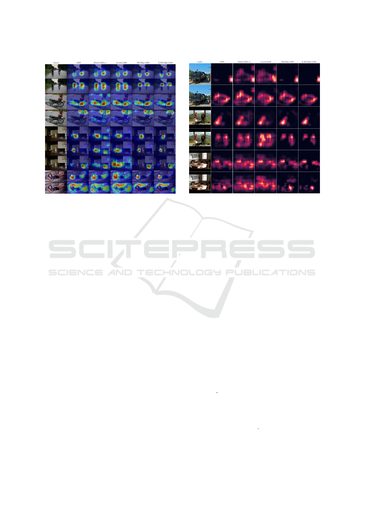
Figure 2: Comparison between CAM-based visualization
techniques over Pascal VOC 2012 dataset. Labels being ex-
plained are, from top to bottom: bicycle, person, motorbike,
person, dining table, chair, tv monitor, person and sofa.
6 IMPROVING VISUALIZATION
While label co-occurrence information might be use-
ful from the classification perspective, handing clues
about the context to the classifier, it provokes unex-
pected highlighting in regions that do not contain the
label. One obvious way to overcome this is to encour-
age solutions that more clearly separate labels and pe-
nalizing the ones that rely on label co-occurrence in-
formation. In this vein, Chan et al. studied the ef-
fect of “balancing” the class distribution of the Deep-
Globe dataset over weakly supervised segmentation,
by removing samples with frequently co-occurring la-
bels, and achieved mixed results (Chan et al., 2021);
while Su et al. proposed a context decoupling strat-
egy based on augmenting samples by pasting objects
outside their usual context (Su et al., 2021).
We propose a regularization strategy that encour-
ages the formation of a positive and sparse synaptic
connection between the signal g = GAP(A
i j
) ∈ R
k
(the output of the last convolutional layer) and the
classifying sigmoid layer. Intuitively, if the presence
of a pattern g
k
is strongly associated with the classi-
fication of a given label c, then g
k
should not be used
in the decision process of the other labels n = C
x
\{c}
(e.g., the presence of a dining table should not con-
tribute to the classification of a chair). Furthermore,
we penalize negative connection values in order to fo-
cus on visual patterns that do characterize the label,
Figure 3: Comparison between CAM-based visualization
techniques over Pascal VOC 2007 dataset. Masks are shown
instead of overlays in order to facilitate visual inspection.
The labels being explained are, from top to bottom: person,
train, motorbike, person, chair, and dining table.
instead of contextual information which indicates its
probable absence (e.g., the absence of a dining table
should not imply absence of chairs).
6.1 Kernel Usage Regularization
Let k be the number of kernels in the last convolu-
tional layer, l be the number of labels in the dataset,
g = [g
i
]
k
be the feature vector obtained from the pool-
ing of last convolutional layer, W = [w
c
i
]
k×l
and b =
[b
c
]
l
the weights from the last dense layer and σ the
sigmoid function. Then, the sigmoid classifier can be
regularized as follows:
W
r
= W ◦ softmax(W )
y = σ(g ·W
r
+ b)
(15)
It is possible to observe that the simple application
of the softmax function over each row in the matrix
W summarizes all of the desired aspects of the regu-
larization: large values w
c
i
(indicating strong connec-
tion between the matching of the pattern described by
kernel i and the classification of label c) will induce
softmax(w
i
)
c
≈ 1, and thus w
c
r
i
≈ w
c
i
. As the softmax
function quickly saturates over a few large values, it
will push the remaining connections towards 0 (eras-
ing the influence kernel i has over the classification of
other labels). Finally, very low (negative) values w
i j
should have low softmax(w
i
)
c
, implying w
c
r
i
≈ 0.
Fig. 4b illustrates the activation maps for the net-
work trained with regularized weights. As the simul-
VISAPP 2022 - 17th International Conference on Computer Vision Theory and Applications
114

taneous usage of same kernels for distinct classifica-
tion units have been regularized, subtracting contribu-
tions no longer distort the maps for any of the labels.
6.2 Results
To demonstrate the efficacy of this strategy, we train
regularized versions of ResNet101 network and com-
pare them with their unregularized counterparts.
In each experiment, we inspected (a) the weight
histograms for each classifying unit in the last layer;
(b) the correlation matrix between the weight vectors
obtained from each unit; and (c) the top-10 most con-
tributing kernels for each of the aforementioned units.
We concluded that (a) most weights have become pos-
itive, as the histograms shifted from a normal-like dis-
tribution centered in zero to a right-skewed-like dis-
tribution; (b) units present a much lower correlation
with each other than the ones observed in their non-
regularized counterparts; and (c) units shared signifi-
cantly less top-10 most contributing kernels.
Table 3 shows the visualization results over mul-
tiple datasets, using a ResNet101 network with a
regularized sigmoid classifier. Once again, Grad-
CAM++ and Score-CAM present high values for
%IC. D-MinMax-CAM shows the best F
1
− scores
in all datasets but one, staying in third place with
a difference of 0.53 percent points from the win-
ner (Score-CAM). Finally, MinMax-CAM and D-
MinMax-CAM showed the best results in 3 out of
4 tests for the F
1
+ score, while achieving a simi-
lar score to the winner (CAM) of the last test (VOC
2007). We observe an overall increase in both In-
crease in Confidence and F
1
+ score for most CAM
techniques and datasets, when compared with their
unregularized counterparts. On the other hand, re-
Table 3: Report of metric scores over multiple datasets, per method. Models were regularized during training.
Metric Dataset CAM Grad-CAM++ Score-CAM MinMax-CAM D-MinMax-CAM
%IC
P:AfS 15.60% 14.39% 14.13% 11.43% 11.54%
COCO 34.43% 36.81% 37.87% 21.47% 21.49%
VOC07 28.71% 28.07% 34.93% 23.90% 24.99%
VOC12 33.32% 34.90% 37.30% 29.54% 29.36%
%AD
P:AfS 42.51% 42.67% 39.50% 51.96% 52.53%
COCO 22.52% 19.86% 13.91% 41.29% 41.39%
VOC07 22.89% 18.65% 11.69% 29.80% 34.19%
VOC12 16.09% 15.32% 10.46% 22.22% 22.85%
%ADO
P:AfS 38.34% 35.46% 35.21% 49.58% 49.51%
COCO 46.97% 37.63% 25.57% 69.17% 69.28%
VOC07 37.30% 20.06% 17.27% 47.16% 48.60%
VOC12 29.66% 21.89% 15.95% 42.07% 42.46%
%AR
P:AfS 47.28% 46.50% 43.61% 43.17% 43.01%
COCO 34.40% 34.21% 28.13% 30.05% 30.04%
VOC07 18.64% 17.35% 16.91% 16.02% 14.72%
VOC12 18.66% 18.37% 17.72% 17.10% 16.99%
%ARO
P:AfS 25.43% 26.35% 26.80% 20.79% 20.72%
COCO 7.14% 7.85% 11.36% 4.24% 4.23%
VOC07 2.44% 3.45% 3.95% 1.35% 1.22%
VOC12 2.59% 2.89% 4.00% 1.22% 1.20%
F
1
−
P:AfS 27.02% 27.68% 26.62% 26.86% 27.15%
COCO 10.08% 10.38% 11.15% 7.33% 7.33%
VOC07 4.12% 5.41% 2.69% 2.47% 2.28%
VOC12 3.97% 4.30% 4.96% 2.24% 2.21%
F
1
+
P:AfS 36.53% 35.05% 34.46% 39.15% 39.03%
COCO 38.08% 34.42% 25.19% 40.64% 40.65%
VOC07 23.89% 17.87% 8.10% 22.38% 20.97%
VOC12 21.99% 19.28% 16.24% 22.84% 22.78%
MinMax-CAM: Improving Focus of CAM-based Visualization Techniques in Multi-label Problems
115

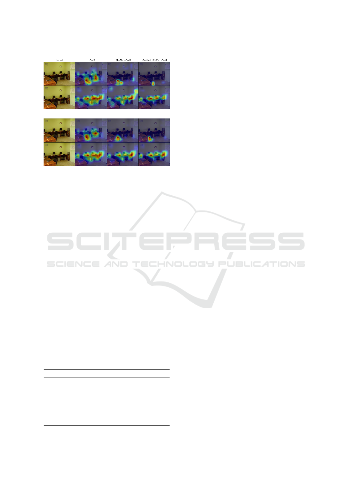
(a)
(b)
Figure 4: (a) Degenerated example in Pascal VOC 2007, in
which contributing regions for the detection of label chair
collide with the ones for label tv monitor. (b) Activation
maps after the network is trained with regularized weights.
sults for F
1
− score were mixed: the value for this
metric has decreased in 9 out of 18 tests. Fur-
thermore, we notice very similar results from both
MinMax-CAM and D-MinMax-CAM in all metrics
and datasets. This can be attributed to the regulariza-
tion factor, which penalizes the existence of negative
weights, approximating max(0, w
c
k
) to w
c
k
and, thus,
D-MinMax-CAM to MinMax-CAM.
Table 4 reports the F
1
and F
2
scores over valida-
tion and test sets (when available) for both baseline
and regularized models. We see a slight increase in
F
1
and F
2
score in most cases, indicating that this
regularization has positive impact on overall score of
the classifier. Conversely, an unexpected decrease in
score was observed for COCO 2017, which might
be associated with its high number of labels and the
training settings used. We hypothesize that a careful
tune of hyperparameters (such as learning rate) can
achieved better results, given the aggressively sparse
nature of this regularization strategy.
Table 4: Multi-label classification score over multiple
datasets, considering the baseline and regularized (Reg.)
models.
Metric Dataset Baseline Reg.
F
2
P:AfS Val 87.80% 88.24%
F
2
P:AfS Priv. Test 89.22% 89.81%
F
2
P:AfS Public Test 89.62% 90.10%
F
1
COCO 2017 Val 75.64% 74.23%
F
1
VOC 2007 Test 84.26% 85.85%
F
1
VOC 2012 Val 85.05% 85.90%
7 CONCLUSIONS
In this work, we promoted an analysis for visualiza-
tion techniques over multi-label scenarios. We pro-
posed generalizations of the well-known Increase in
Confidence and Average Drop metrics, accounting for
the multiple labels within each sample, and presented
three new metrics that capture the effectiveness of vi-
sualization maps in images containing objects of dis-
tinct labels. We found existing techniques, focused
solely on optimizing Increase in Confidence and Av-
erage Drop, to produce diffuse maps.
We presented a visualization technique that pro-
duces visualization maps considering the activation
maximization for a labels of interest while minimiz-
ing the activation of adjacent labels. We further re-
fined this technique by decomposing it into posi-
tive, negative and background contributions in order
to produce cleaner visualization maps with minimal
contextual residue. We tested our solutions over dif-
ferent datasets and architectures, obtaining encourag-
ing results from the multiple metrics while maintain-
ing low processing footprint (compared to the mas-
sively time consuming Score-CAM).
Finally, we proposed a regularization strategy
which penalizes the usage of label co-occurrence in-
formation in the classification process by reinforcing
positive and sparse weights in the classification layer.
Quantitative results suggest that this strategy is effec-
tive in creating cleaner visualization maps while pro-
moting better classification scores in most datasets.
Future work will include an evaluation of our tech-
nique over localization and weakly supervised seg-
mentation problems, as well as the development of
a generalized kernel usage regularization strategy that
can extended to intermediate layers. Furthermore, we
intent to study new ways to decouple label contextual
information by distilling label-specific knowledge.
ACKNOWLEDGEMENTS
The authors would like to thank CNPq (grants
140929/2021-5 and 309330/2018-1) and
LNCC/MCTI for providing HPC resources of
the SDumont supercomputer.
REFERENCES
Adebayo, J., Gilmer, J., Muelly, M., Goodfellow, I.,
Hardt, M., and Kim, B. (2018). Sanity checks for
saliency maps. In 32nd International Conference on
Neural Information Processing Systems (NIPS), page
VISAPP 2022 - 17th International Conference on Computer Vision Theory and Applications
116

9525–9536, Red Hook, NY, USA. Curran Associates
Inc.
Chan, L., Hosseini, M. S., and Plataniotis, K. N. (2021).
A comprehensive analysis of weakly-supervised se-
mantic segmentation in different image domains.
International Journal of Computer Vision (IJCV),
129(2):361–384.
Chattopadhay, A., Sarkar, A., Howlader, P., and Balasub-
ramanian, V. N. (2018). Grad-CAM++: Generalized
gradient-based visual explanations for deep convolu-
tional networks. In IEEE Winter Conference on Appli-
cations of Computer Vision (WACV), pages 839–847.
IEEE.
Dhillon, A. and Verma, G. K. (2020). Convolutional neu-
ral network: a review of models, methodologies and
applications to object detection. Progress in Artificial
Intelligence, 9(2):85–112.
Everingham, M., Van Gool, L., Williams, C. K., Winn,
J., and Zisserman, A. (2010). The pascal visual ob-
ject classes (voc) challenge. International Journal of
Computer Vision (IJCV), 88(2):303–338.
Huff, D. T., Weisman, A. J., and Jeraj, R. (2021). Interpre-
tation and visualization techniques for deep learning
models in medical imaging. Physics in Medicine &
Biology, 66(4):04TR01.
Lee, J. R., Kim, S., Park, I., Eo, T., and Hwang, D. (2021).
Relevance-CAM: Your model already knows where
to look. In IEEE/CVF Conference on Computer Vi-
sion and Pattern Recognition (CVPR), pages 14944–
14953.
Lin, T.-Y., Maire, M., Belongie, S., Hays, J., Perona, P.,
Ramanan, D., Doll
´
ar, P., and Zitnick, C. L. (2014).
Microsoft coco: Common objects in context. In Fleet,
D., Pajdla, T., Schiele, B., and Tuytelaars, T., editors,
European Conference on Computer Vision (ECCV),
pages 740–755, Cham. Springer International Pub-
lishing.
Minaee, S., Boykov, Y. Y., Porikli, F., Plaza, A. J., Kehtar-
navaz, N., and Terzopoulos, D. (2021). Image seg-
mentation using deep learning: A survey. IEEE Trans-
actions on Pattern Analysis and Machine Intelligence
(PAMI), pages 1–1.
Pons, J., Slizovskaia, O., Gong, R., G
´
omez, E., and Serra,
X. (2017). Timbre analysis of music audio signals
with convolutional neural networks. In 25th Eu-
ropean Signal Processing Conference (EUSIPCO),
pages 2744–2748. IEEE.
Ramaswamy, H. G. et al. (2020). Ablation-CAM: Vi-
sual explanations for deep convolutional network via
gradient-free localization. In IEEE/CVF Winter Con-
ference on Applications of Computer Vision (WACV),
pages 983–991.
Rawat, W. and Wang, Z. (2017). Deep convolutional neural
networks for image classification: A comprehensive
review. Neural Computation, 29(9):2352–2449.
Selvaraju, R. R., Cogswell, M., Das, A., Vedantam, R.,
Parikh, D., and Batra, D. (2017). Grad-CAM: Visual
explanations from deep networks via gradient-based
localization. In IEEE International Conference on
Computer Vision (ICCV), pages 618–626.
Shendryk, I., Rist, Y., Lucas, R., Thorburn, P., and Tice-
hurst, C. (2018). Deep learning - a new approach
for multi-label scene classification in planetscope and
sentinel-2 imagery. In IEEE International Geoscience
and Remote Sensing Symposium (IGARSS), pages
1116–1119.
Simonyan, K., Vedaldi, A., and Zisserman, A. (2014).
Deep inside convolutional networks: Visualising im-
age classification models and saliency maps. CoRR,
abs/1312.6034.
Smilkov, D., Thorat, N., Kim, B., Vi
´
egas, F. B., and Wat-
tenberg, M. (2017). SmoothGrad: removing noise by
adding noise. ArXiv, abs/1706.03825.
Springenberg, J., Dosovitskiy, A., Brox, T., and Riedmiller,
M. (2015). Striving for simplicity: The all convolu-
tional net. In International Conference on Learning
Representations (ICLR) - Workshop Track.
Srinivas, S. and Fleuret, F. (2019). Full-gradient represen-
tation for neural network visualization. arXiv preprint
arXiv:1905.00780.
Su, Y., Sun, R., Lin, G., and Wu, Q. (2021). Context de-
coupling augmentation for weakly supervised seman-
tic segmentation. ArXiv, abs/2103.01795.
Tachibana, H., Uenoyama, K., and Aihara, S. (2018). Effi-
ciently trainable text-to-speech system based on deep
convolutional networks with guided attention. In
IEEE International Conference on Acoustics, Speech
and Signal Processing (ICASSP), pages 4784–4788.
Tarekegn, A. N., Giacobini, M., and Michalak, K. (2021).
A review of methods for imbalanced multi-label clas-
sification. Pattern Recognition, 118:107965.
Wang, H., Wang, Z., Du, M., Yang, F., Zhang, Z., Ding, S.,
Mardziel, P., and Hu, X. (2020). Score-CAM: Score-
weighted visual explanations for convolutional neural
networks. IEEE/CVF Conference on Computer Vision
and Pattern Recognition Workshops (CVPRW), pages
111–119.
Wei, S.-E., Ramakrishna, V., Kanade, T., and Sheikh, Y.
(2016). Convolutional pose machines. In IEEE con-
ference on Computer Vision and Pattern Recognition
(CVPR), pages 4724–4732.
Yao, L., Mao, C., and Luo, Y. (2019). Graph convolu-
tional networks for text classification. In AAAI con-
ference on artificial intelligence, volume 33, pages
7370–7377.
Zhang, D., Han, J., Cheng, G., and Yang, M.-H. (2021).
Weakly supervised object localization and detection:
A survey. IEEE Transactions on Pattern Analysis and
Machine Intelligence, pages 1–1.
Zhou, B., Khosla, A., Lapedriza, A., Oliva, A., and Tor-
ralba, A. (2016). Learning deep features for discrimi-
native localization. In IEEE Conference on Computer
Vision and Pattern Recognition (CVPR), pages 2921–
2929.
MinMax-CAM: Improving Focus of CAM-based Visualization Techniques in Multi-label Problems
117