DAEs for Linear Inverse Problems: Improved Recovery with Provable

Guarantees

Jasjeet Dhaliwal and Kyle Hambrook

Department of Mathematics, San Jose State University, San Jose, U.S.A.

Keywords:

Autoencoders, Generative Priors, Compressive Sensing, Inpainting, Superresolution.

Abstract:

Generative priors have been shown to provide improved results over sparsity priors in linear inverse prob-

lems. However, current state of the art methods suffer from one or more of the following drawbacks: (a)

speed of recovery is slow; (b) reconstruction quality is deﬁcient; (c) reconstruction quality is contingent on a

computationally expensive process of tuning hyperparameters. In this work, we address these issues by utiliz-

ing Denoising Auto Encoders (DAEs) as priors and a projected gradient descent algorithm for recovering the

original signal. We provide rigorous theoretical guarantees for our method and experimentally demonstrate

its superiority over existing state of the art methods in compressive sensing, inpainting, and super-resolution.

We ﬁnd that our algorithm speeds up recovery by two orders of magnitude (over 100x), improves quality of

reconstruction by an order of magnitude (over 10x), and does not require tuning hyperparameters.

1 INTRODUCTION

Linear inverse problems can be formulated mathemat-

ically as y = Ax+e where y ∈ R

is the observed vec-

tor, A ∈ R

m×N

is the measurement process, e ∈ R

a noise vector, and x ∈ R

is the original signal. The

problem is to recover the signal x, given the obser-

vation y and the measurement matrix A. Such prob-

lems arise naturally in a wide variety of ﬁelds includ-

ing image processing, seismic and medical tomogra-

phy, geophysics, and magnetic resonance imaging. In

this paper, we focus on three linear inverse problems

encountered in image processing: compressive sens-

ing, inpainting, and super-resolution. We motivate

our method using the compressive sensing problem.

Sparsity Prior. The problem of compressive sensing

assumes the matrix A ∈ R

m×N

is fat, i.e. m < N. Even

when no noise is present (y = Ax), the system is under

determined and the recovery problem is intractable.

However, it has been shown that if the matrix A satis-

ﬁes certain conditions such as the Restricted Isometry

Property (RIP) and if x is known to be approximately

sparse in some ﬁxed basis, then x can typically be re-

covered even when m  N (Tibshirani, 1996; Donoho

et al., 2006; Candes et al., 2006).

Sparsity (or approximate sparsity) is a very

restrictive condition to impose on the signal as it

limits the applicability of recovery methods to a small

subset of input domains. There has been considerable

effort in using other forms of structured priors such

as structured sparsity (Baraniuk et al., 2010), sparsity

in tree-structured dictionaries (Peyre, 2010), and

low-rank mixture of Gaussians (Chen et al., 2010).

Although these efforts improve on the sparsity prior,

they do not cater to signals that are not naturally

sparse or structured-sparse.

Generative Prior. Bora et al. (Bora et al., 2017) ad-

dress this issue by replacing the sparsity prior on x

with a generative prior. In particular, the authors ﬁrst

train a generative model f : R

7→ R

with k < N that

maps a lower dimensional latent space to the higher

dimensional ambient space. This model is referred

to as the generator. Next, they impose the prior that

the original signal x lies in (or near) the range of f .

Hence, the recovery problem reduces to ﬁnding the

best approximation to x in f (R

The quality of the generative prior depends on

how well the training set captures the data dis-

tribution. Bora et al.(Bora et al., 2017) used a

Generative Adversarial Network (GAN) as the gen-

erator, G : R

7→ R

, where k < N, to model

the distribution of the training data and posed the

following non-convex optimization problem ˆz =

arg min

z∈R



kAG(z) − yk

+ λkzk



. such that G(ˆz) is

We use

to denote the `

-norm throughout the paper

Dhaliwal, J. and Hambrook, K.

DAEs for Linear Inverse Problems: Improved Recovery with Provable Guarantees.

DOI: 10.5220/0010804500003124

In Proceedings of the 17th International Joint Conference on Computer Vision, Imaging and Computer Graphics Theory and Applications (VISIGRAPP 2022) - Volume 4: VISAPP, pages

97-105

ISBN: 978-989-758-555-5; ISSN: 2184-4321

Figure 1: CS on CelebA without noise for m = 1000 (left), CS on CelebA with noise for m = 1000 (middle), CS on CelebA for

various m using DAE-PGD (right). The left and middle images qualitatively capture the 10x improvement in reconstruction

error. The right image shows how DAE-PGD reconstructions capture ﬁner grained details as m increases.

treated as the approximation to x. The authors pro-

vided recovery guarantees for their methods and vali-

dated the efﬁcacy of using generative priors by show-

ing that their method required 5-10x fewer measure-

ments than Lasso (with a sparsity constraint) (Tibshi-

rani, 1996) while yielding the same accuracy in re-

covery. However, since the problem is non-convex

and requires a search over R

, it is computationally

expensive and the reconstruction quality depends on

the initialization vector z ∈ R

Since then, there have been signiﬁcant efforts to

improve recovery results using neural networks as

generative priors (Adler and

Oktem, 2017; Fan et al.,

2017; Gupta et al., 2018; Liu et al., 2017; Mardani

et al., 2018; Metzler et al., 2017; Mousavi et al.,

2017; Rick Chang et al., 2017a; Shah and Hegde,

2018; Yeh et al., 2017; Raj et al., 2019; Heckel and

Hand, 2018). Shah et al. (Shah and Hegde, 2018)

extended the work of (Bora et al., 2017) by train-

ing a generator G and using a projected gradient de-

scent algorithm that consists of a gradient descent step

= x

− ηA

(Ax

− y) followed by a projection step

t+1

= G(arg min

z∈R

kG(z) − w

)The core idea being

that the estimate w

is improved by projecting it onto

the range of G. However, since their method requires

solving a non-convex optimization problem at every

update step, it also leads to slow recovery.

Raj et al. (Raj et al., 2019) enhanced the results

of (Shah and Hegde, 2018) by eliminating the expen-

sive non-convex optimization based projection step

with one that is an order of magnitude cheaper. In

particular, they trained a GAN G to model the data

distribution and also trained a pseudo-inverse GAN

‡

that learned a mapping from the ambient space to

the latent space. Next, they used the projection step:

t+1

= G(G

‡

)). By eliminating the need to solve a

non-convex optimization problem to update x

t+1

, they

were able to attain a signiﬁcant speed up in the run-

ning time of the recovery algorithm.

However, the recovery algorithm of (Raj et al.,

2019) has two main drawbacks. First, training two

networks: G and G

‡

makes the training process and

the projection step unnecessarily convoluted. Second,

their recovery guarantees only hold when the learning

rate η =

, where β is a RIP-style constant of the

matrix A. Since it is NP-hard to estimate the constant

β (Bandeira et al., 2013), it follows that setting η =

is NP-hard as well.

DAE Prior. In an effort to address the aforemen-

tioned issues, we propose to use a DAE (Vincent

et al., 2008) prior in lieu of the generative prior in-

troduced by Bora et al. (Bora et al., 2017). It

has previously been shown that DAEs not only cap-

ture useful structure of the data distribution (Vincent

et al., 2010) but also implicitly capture properties of

the data-generating density (Alain and Bengio, 2014;

Bengio et al., 2013). Moreover, as DAEs are trained

to remove noise from vectors sampled from the input

distribution, they integrate naturally with gradient de-

scent algorithms that lead to noisy approximations at

each time step.

We replace the generator G used in Bora et al.

(Bora et al., 2017) with a DAE F : R

7→ R

such

that the range of F contains the vectors from the orig-

inal data generating distribution. We then impose the

prior that the original signal x lies in the range of F

and utilize Algorithm 1 to recover an approximation

to x. We provide theoretical recovery guarantees and

ﬁnd that our framework speeds up recovery by two

orders of magnitude (over 100x), improves quality of

reconstruction by an order of magnitude (over 10x),

and does not require tuning hyperparameters. We note

that Peng et al. (Peng et al., 2020) have recently uti-

lized Auto Encoders (AE) instead of DAEs as in our

We observed this problem when trying to reproduce the

experimental results of (Raj et al., 2019). Speciﬁcally, we

tried an exhaustive grid-search for η but each value led to

poor reconstruction quality.

VISAPP 2022 - 17th International Conference on Computer Vision Theory and Applications

approach. However, unlike our work, their theoretical

results rely on the measurement matrix being Gaus-

sian and we ﬁnd their experimental results are inferior

to those of Algorithm 1 (Section 3.2).

2 ALGORITHM AND RESULTS

2.1 Denoising Auto Encoder

A DAE is a non-linear mapping F : R

7→ R

that

can be written as a composition of two non-linear

mappings - an encoder E : R

7→ R

where k < N

and a decoder D : R

7→ R

. Therefore, F(x) =

(D ◦ E)(x). Given a set of n samples from a domain

of interest {x

}

i=1

, the training set X is created by

adding Gaussian noise to the original samples. That

is, X = {x

}

i=1

, where x

= x

and e

∼ N (µ

, σ

The loss function for training F is the Mean

Squared Error (MSE) loss deﬁned as : L

(X) =

∑

i=1

kF(x

) − x

. The training procedure uses

gradient descent to minimize L

(X) with back-

propagation.

2.2 Algorithm

Recall that in the linear inverse problem y = Ax + e,

our goal is to recover an approximation ˆx to x such

that ˆx lies in the range of F. Thus we aim to ﬁnd

ˆx such that ˆx = arg min

z∈F(R

)

kAz − yk

As in (Shah and

Hegde, 2018; Raj et al., 2019), we use a projected

gradient descent algorithm. Given an estimate x

at it-

eration t, we compute a gradient descent step for solv-

ing the unrestricted problem: minimize

z∈R

kAz − yk

as:

← x

− ηA

(Ax

− y) Next we project w

onto the

range of F to satisfy our prior: x

t+1

= F(w

) Note

that, compared to (Shah and Hegde, 2018; Raj et al.,

2019), the projection step does not require solving a

non-convex optimization problem.

Now suppose that the domain of interest is rep-

resented by the set D ⊆ R

. Then, given a vector

= x + e, where x ∈ D, and e ∈ R

is an unknown

noise vector, the success of our method depends on

how small the error kF(x

)−xk is. If the training set X

captures the domain of interest well and if the training

procedure utilizes a diverse enough set of noise vec-

tors {e

}

i=1

, then we expect kF(x

) − xk to be small.

Consequently, we expect the projection step of Algo-

rithm 1 to yield vectors in or close to D. We provide

the complete algorithm below.

Algorithm 1: DAE-PGD.

Input: y ∈ R

,A ∈ R

m×N

, f : R

→ R

T ∈ Z

,η ∈ R

Output: x

1: t ← 0, x

← 0

2: while t < T do

3: w

← x

− ηA

(Ax

− y)

4: x

t+1

← f (w

)

5: return x

2.3 Theoretical Results

We begin by introducing two standard deﬁnitions re-

quired to provide recovery guarantees.

Deﬁnition 1 (RIP(S,δ)). Given S ⊆ R

and δ > 0, a

matrix A ∈ R

m×N

satisﬁes the RIP(S,δ) property if

(1−δ)

− x

≤

A(x

− x

)

≤ (1+δ)

− x

for all x

∈ S.

A variation of the RIP(S,δ) property for sparse

vectors was ﬁrst introduced by Candes et al. in (Can-

des and Tao, 2005) and has been shown to be a suf-

ﬁcient condition in proving recovery guarantees us-

ing `

-minimization methods (Foucart and Rauhut,

2017). Next, we deﬁne an Approximate Projection

(AP) property and provide an interpretation that elu-

cidates its role in the results of Theorem 6.

Deﬁnition 2 (AP(S, α)). Let α ≥ 0. A mapping

f : R

→ S ⊆ R

satisﬁes AP(S,α) if

w − f (w)

≤ kw − xk

+ αk f (w) − xk

for every w ∈ R

and x ∈ S.

We now explain the signiﬁcance of Def. 5. Let

∗

= arg min

z∈S

w − z

and observe

w − f (w)

≤ (

w − x

∗

f (w) − x

∗

)

(1)

Hence, α ≤

f (w) − x

∗

w − x

∗

is needed to en-

sure the RHS of Def. 5 is bounded by the RHS of

(1). In other words, for α to be small, the projec-

tion error

f (w) − x

∗

as well as distance of w to S

need to be small. Since the DAE F learns to mini-

mize

F(w) − x

∗

(Section 2.1), we expect a small

projection error.

Theorem 3. Let f : R

→ S ⊆ R

satisfy AP(S, α)

and let A ∈ R

m×N

be a matrix with kAk

≤ M that

Various ﬂavors of the AP(S,α) property have been used

in previous works, such as Shah et al. (Shah and Hegde,

2018) and Raj et al. (Raj et al., 2019).

DAEs for Linear Inverse Problems: Improved Recovery with Provable Guarantees

satisﬁes RIP(S, δ). If y = Ax with x ∈ S, the recovery

error of Algorithm 1 is bounded as:

− x

≤ (2γ)

− x

+ α



1 − (2γ)



(2)

where γ =

M(1 + δ) + 2η(δ − 1) + 1.

Theorem 6 tells us that, if γ <

, then for large T ,

the recovery error is essentially α/(1 −2γ). Note that

the requirement γ <

is satisﬁed for a large range of

values of η as long as δ is sufﬁciently small

. Hence,

as long as the value of α is small, we expect to see a

small recovery error.

We now compare the above results to Theorem 1

of (Raj et al., 2019), Theorem 2.2 of (Shah and Hegde,

2018) and Theorem 1 of (Peng et al., 2020). As men-

tioned in Section 1, convergence in Theorem 1 of (Raj

et al., 2019) is only guaranteed when η =

, which is

a much more restrictive condition on η than Theorem

6 provides. In fact, β is a RIP-style constant that is

NP-hard to ﬁnd (Bandeira et al., 2013) which makes

setting the value of η =

NP-hard as well. The re-

sults of Theorem 2.2 from (Shah and Hegde, 2018)

require a less restrictive constraint on η but do re-

quire a stricter constraint on

≤ ω, where ω is

a RIP-style constant for A. In contrast, the results of

Theorem 6 do not impose a strict condition on

Finally, the proof of Theorem 1 of (Peng et al., 2020)

relies on the matrix A being Gaussian. We do not im-

pose such a constraint.

3 EXPERIMENTS

We provide experimental results for the problems

of compressive sensing, inpainting, and super-

resolution. We refer to the results of Algorithm 1 as

DAE-PGD and compare its results to the methods of

Bora et al. (Bora et al., 2017) ( CSGM), and Shah et

al. (Shah and Hegde, 2018), ( PGD-GAN), and Peng

et al (Peng et al., 2020) (P-AE). Although the work

of Raj et al. (Raj et al., 2019) is the closest to our

method, we do not include comparisons to their work

as we were unable to reproduce their results

For instance, random Gaussian matrices yield small

values for δ with high probability (Foucart and Rauhut,

2017)

We used their code, their trained models, their recovery

algorithm, and a grid search for η but the reconstructed im-

ages were of very poor quality. We also reached out to the

authors but they did not have the exact values of η that were

used in their experiments.

3.1 Setup

Datasets. Our experiments are conducted on the

MNIST (LeCun, ) and CelebA (Liu et al., 2015)

datasets. The MNIST dataset consists of 28 × 28

greyscale images of digits with 50,000 training

and 10,000 test samples. We report results for a

random subset of the test set. The CelebA dataset

consists of more than 200,000 celebrity images. We

pre-processes each image to a size of 64×64 × 3 and

use the ﬁrst 160, 000 images as the training set and a

random subset of the remaining 40,000+ images as

the test set.

Network Architecture. The network architectures

for our DAEs are inspired by the Variational Auto

Encoder architecture from Fig 2. of (Hou et al., 2017)

with a few key changes. We replace the Leaky Relu

activation with Relu, we add the two outputs of the

encoder to get the latent representation z, and we alter

the kernel sizes as well as the convolution strides of

the network as described in the Appendix.

Training. We use the Adam optimizer (Kingma and

Ba, 2014) to minimize the MSE loss function with

learning rate 0.01 and a batch size of 128. We train

the CelebA network for 400 epochs and the MNIST

network for 100 epochs.

In an effort to ensure that kA(x

) − xk deﬁned in

Section 2.2 is small, we split the training set into

5 equal sized subsets. For each distinct subset, we

sample the noise vectors from a Gaussian distribution

N (µ, σ

) with a distinct value for σ for each sub-

set. The ﬁve different values for σ that we use are

{0.25,0.5, 0.75,1.0,1.25}.

All of our experiments were conducted on a Tesla

M40 GPU with 12 GB of memory using Keras (Chol-

let, 2015) and Tensorﬂow (Abadi et al., 2015) li-

braries. The code to reproduce our results is available

here.

3.2 Compressive Sensing

We consider the problem of compressive sensing

without noise: y = Ax and with noise: y = Ax + e,

with e ∼ N (0,0.25). We use m to denote the num-

ber of observed measurements in our results (i.e. y ∈

). As done in previous works (Bora et al., 2017;

Shah and Hegde, 2018; Raj et al., 2019), the matrix

A ∈ R

m×N

is chosen to be a random Gaussian ma-

trix with A

i j

∼ N (0,

). Finally, we set the learning

rate of Algorithm 1 as η = 1. Note that in both (with

and w/out noise) cases, we also include recovery re-

sults for the Lasso algorithm (Tibshirani, 1996) with

a DCT basis (L-DCT) and with a wavelet basis (L-

VISAPP 2022 - 17th International Conference on Computer Vision Theory and Applications

100

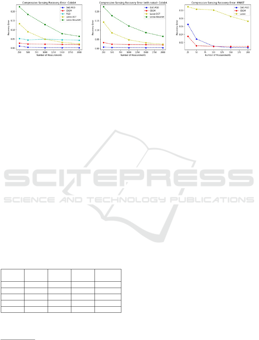
Figure 2: Compressive Sensing recovery error:

x − ˆx

. Left: CelebA without noise - DAE-PGD shows over 10x improve-

ment. Middle: CelebA with noise - DAE-PGD shows over 10x improvement. Right: MNIST without noise - DAE-PGD beats

CSGM for m > 100.

Wavelet).

We begin with CelebA. Figure 1 provides a qual-

itative comparison of reconstruction results for m =

1000. We observe that DAE-PGD provides the best

quality reconstructions and is able to reproduce even

ﬁne grained details of the original images such as

eyes, nose, lips, hair, texture, etc. Indeed the high

quality reconstructions support the case that the DAE

has a small α as per Def. 5. For a quantitative com-

parison, we turn to Figure 2 which plots the average

squared reconstruction error kx − ˆxk

for each algo-

rithm at different values of m. Note that DAE-PGD

provides more than 10x improvement in the squared

reconstruction error.

In order to capture how the quality of reconstruc-

tion degrades as the number of measurements de-

crease, we refer to Figure 1, which shows reconstruc-

tions for different values of m. We observe that even

though reconstructions with a small number of mea-

surements capture the essence of the original images,

the ﬁne grained details are captured only as the num-

ber of measurements increase.

We show a similar comparison for MNIST in Fig-

ure 3

Table 1: Average running times (in seconds) for the Com-

pressive Sensing problem (w/out noise) on the CelebA

dataset.

m CGSM

PGD-

GAN

DAE-

PGD

Speedup

250 53.78 48.40 0.07 692x

500 59.81 48.46 0.09 538x

1000 81.08 48.46 0.11 440x

1500 92.68 48.50 0.14 346x

2000 107.41 48.56 0.21 230x

We now turn to the speed of reconstruction. Table

1 shows that our method provides speedups of over

100x as compared to PGD-GAN and CSGM

CSGM is executed for 500 max iterations with 2

restarts and PGD-GAN is executed for 100 max iterations

and 1 restart.

3.3 Inpainting

Inpainting is the problem of recovering the original

image, given an occluded version of it. Speciﬁcally,

the observed image y consists of occluded (or masked

) regions created by applying a pixel-wise mask A to

the original image x. We use m to refer to the size

of mask that occludes a m × m region of the original

image x.

We present recovery results for CelebA with m =

10 in Figure 4 and observe that DAE-PGD is able to

recovery a high quality approximation to the original

image and outperforms CSGM in all cases. Figure

4 also captures how recovery is affected by different

mask sizes. As in the compressive sensing problem,

we ﬁnd that DAE-PGD reconstructions capture the

ﬁne-grained details of each image. Figure 4 also re-

ports the result for the MNIST dataset. Even though

DAE-PGD outperforms CSGM, we see that the re-

covery quality of DAE-PGD degrades considerably

when m = 15. We hypothesize this is due to the struc-

ture of MNIST images. In particular, since MNIST

images are grayscale with most of the pixels being

black, putting a 15 × 15 black patch on the small area

displaying the number makes the reconstruction prob-

lem considerably more difﬁcult. This causes consid-

erable degradation in reconstruction quality for larger

mask sizes.

3.4 Super-resolution

Super-resolution is the problem of recovering the

original image from a smaller and lower-resolution

version. We create this smaller and lower-resolution

image by taking the spatial averages of f × f pixel

values where f is the ratio of downsampling. This re-

sults in blurring a f × f region followed by downsam-

pling the image. We test our algorithm with f = 2,3,4

corresponding to 4×,9×, and 16× smaller image

sizes, respectively.

DAEs for Linear Inverse Problems: Improved Recovery with Provable Guarantees

101

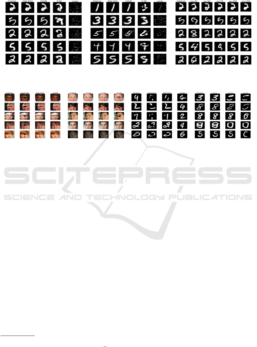
Figure 3: CS on MNIST without noise for m = 100 (left), CS on MNIST with noise for m = 100 (middle), CS on CelebA for

various m using DAE-PGD (right). The left and middle images qualitatively capture the 100x improvement in reconstruction

error. The right image shows how DAE-PGD reconstructions capture ﬁner grained details as m increases.

Figure 4: Inpainting. Left: CelebA reconstructions for m = 10. Middle-Left: DAE-PGD CelebA reconstructions for different

m. Middle-Right: MNIST reconstructions for m = 5. Right: DAE-PGD MNIST reconstructions for different m.

The reconstruction results are provided in 5. We

see that DAE-PGD provides higher quality recon-

struction for f = 2 for both CelebA and MNIST.

Moreover, reconstruction quality degrades gracefully

for CelebA for increasing values of f . However, in the

case of MNIST, reconstruction quality degrades con-

siderably when f = 4. Noting that f = 4 only gives

16 measurements (i.e. y ∈ R

), we hypothesize that

16 measurements may not contain enough signal

accurately reconstruct the original images.

4 RELATED WORK

Compressive Sensing. The ﬁeld of compressive

sensing was initiated with the work of (Cand

es et al.,

2006) and (Donoho et al., 2006) where provided

recovery results for sparse signals with a random

measurement matrix. Some of the earlier work in

extending compressive sensing to perform stable

recovery with deterministic matrices was done

by (Candes and Tao, 2005) and (Candes et al.,

2006), where a sufﬁcient condition for recovery

was satisfaction of a restricted isometry hypothesis.

(Blumensath and Davies, 2009) introduced IHT as

an algorithm to recover sparse signals which was

Consider compressive sensing with sparsity constraints

where recovery guarantees hold when m ≥ Cs ln(

) (Fou-

cart and Rauhut, 2017).

later modiﬁed in (Baraniuk et al., 2010) to reduce

the search space as long as the sparsity was structured.

Generative Priors. Following the lead of (Bora

et al., 2017), there have been signiﬁcant efforts to

improve on previous recovery results using neural

networks as generative models (Adler and

Oktem,

2017; Fan et al., 2017; Gupta et al., 2018; Liu et al.,

2017; Mardani et al., 2018; Metzler et al., 2017;

Mousavi et al., 2017; Rick Chang et al., 2017a;

Shah and Hegde, 2018; Yeh et al., 2017; Raj et al.,

2019; Heckel and Hand, 2018). One line of work

(Jagatap and Hegde, 2019; Heckel and Hand, 2018)

extends the efforts of Bora et al. (Bora et al., 2017)

by ﬁxing a seed z and ﬁnding the weights ˆw of

an untrained neural network G in the optimization

problem ˆw = arg min

w∈R

kAG(w,z) − yk

. However,

the optimization problem is highly non-convex and

requires a large number of iterations with multiple

restarts. Another line of work, (Mousavi et al., 2017;

Mousavi and Baraniuk, 2017) trains a neural network

to model the transformation f (y) = ˆx where ˆx is the

approximation to the original input x. This approach

is limited as a) the inverse mapping is non-trivial to

learn and b) will only work for a ﬁxed measurement

mechanism.

Denoisers in Linear Inverse Problems. Given

the success of denoisers in image processing tasks

such as image denoising (Wang et al., 2018; Guo

VISAPP 2022 - 17th International Conference on Computer Vision Theory and Applications

102

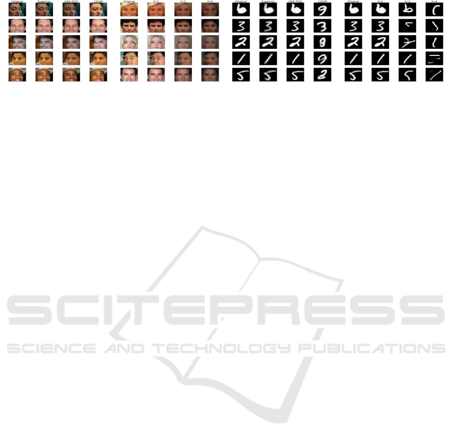
Figure 5: Super-resolution. Left: CelebA reconstructions for f = 2. Middle-Left: DAE-PGD CelebA reconstructions for

different f . Middle-Right: MNIST reconstructions for f = 2. Right: DAE-PGD MNIST reconstructions for different f .

et al., 2019; Rick Chang et al., 2017b) and im-

age super-resolution (Sønderby et al., 2016) to yield

good results, (Venkatakrishnan et al., 2013) intro-

duced denoisiers as plug-and-play (PnP) proximal op-

erators in solving linear inverse problems via alternat-

ing directions method of multipliers (ADMM). (Ryu

et al., 2019) extended this work by investigating con-

vergence properties of ADMM methods asked and

showed that if the denoiser was close to the identity

map, then PnP methods are contractive iterations that

converge with bounded error.

(Rick Chang et al., 2017b) showed that neural net-

work based denoisers (such as DAEs) with ADMM

could achieve state of the art results for a wide ar-

ray of linear inverse problems. They also showed

that if the gradient of the proximal operator (de-

noiser) is Lipschitz continuous, ADMM has a ﬁxed

point. (Xu et al., 2020) analyzed convergence results

for minimum mean squared error (MMSE) denois-

ers used in iterative shrinkage/thresholding algorithm

(ISTA). They showed that the iterates produced by

ISTA with an MMSE denoiser converge to a station-

ary point of some global cost function. (Meinhardt

et al., 2017) demonstrated that using a ﬁxed denoising

network as a proximal operator in the primal-dual hy-

brid gradient (PDHG) method yields state-of-the-art

results. (Gonz

alez et al., 2021) used variational auto

encoders (VAEs) as priors deﬁned an optimization

method JPMAP that performs Joint Posterior Maxi-

mization using an the VAE prior. They showed the-

oretical and experimental evidence that the proposed

objective function satisﬁes a weak bi-convexity prop-

erty which is sufﬁcient to guarantee that the optimiza-

tion scheme converges to a stationary point.

5 CONCLUSION

We introduced DAEs as priors for general linear in-

verse problems and provided experimental results for

the problems of compressive sensing, inpainting, and

super-resolution on the CelebA and MNIST datasets.

Utilizing a projected gradient descent algorithm for

recovery, we provided rigorous theoretical guarantees

for our framework and showed that our recovery algo-

rithm does not impose strict constraints on the learn-

ing rate and hence eliminates the need to tune hy-

perparameters. We compared our framework to state

of the art methods experimentally and found that our

recovery algorithm provided a speed up of over two

orders of magnitude and an order of magnitude im-

provement in reconstruction quality.

REFERENCES

Abadi, M., Agarwal, A., Barham, P., Brevdo, E., Chen, Z.,

Citro, C., Corrado, G. S., Davis, A., Dean, J., Devin,

M., Ghemawat, S., Goodfellow, I., Harp, A., Irving,

G., Isard, M., Jia, Y., Jozefowicz, R., Kaiser, L., Kud-

lur, M., Levenberg, J., Man

e, D., Monga, R., Moore,

S., Murray, D., Olah, C., Schuster, M., Shlens, J.,

Steiner, B., Sutskever, I., Talwar, K., Tucker, P., Van-

houcke, V., Vasudevan, V., Vi

egas, F., Vinyals, O.,

Warden, P., Wattenberg, M., Wicke, M., Yu, Y., and

Zheng, X. (2015). TensorFlow: Large-scale machine

learning on heterogeneous systems. Software avail-

able from tensorﬂow.org.

Adler, J. and

Oktem, O. (2017). Solving ill-posed inverse

problems using iterative deep neural networks. In-

verse Problems, 33(12):124007.

Alain, G. and Bengio, Y. (2014). What regularized

auto-encoders learn from the data-generating distri-

bution. The Journal of Machine Learning Research,

15(1):3563–3593.

Bandeira, A. S., Dobriban, E., Mixon, D. G., and Sawin,

W. F. (2013). Certifying the restricted isometry prop-

erty is hard. IEEE transactions on information theory,

59(6):3448–3450.

Baraniuk, R. G., Cevher, V., Duarte, M. F., and Hedge,

C. (2010). Model-based compressive sensing. IEEE

Transactions on Information Theory, 56(4):1982–

2001.

Bengio, Y., Yao, L., Alain, G., and Vincent, P. (2013). Gen-

eralized denoising auto-encoders as generative mod-

els. Advances in neural information processing sys-

tems, 26:899–907.

Blumensath, T. and Davies, M. E. (2009). Iterative hard

thresholding for compressed sensing. Applied and

computational harmonic analysis, 27(3):265–274.

DAEs for Linear Inverse Problems: Improved Recovery with Provable Guarantees

103

Bora, A., Jalal, A., Price, E., and Dimakis, A. G. (2017).

Compressed sensing using generative models. arXiv

preprint arXiv:1703.03208.

Candes, E. and Tao, T. (2005). Decoding by linear program-

ming. arXiv preprint math/0502327.

Cand

es, E. J., Romberg, J., and Tao, T. (2006). Ro-

bust uncertainty principles: Exact signal reconstruc-

tion from highly incomplete frequency information.

IEEE Transactions on information theory, 52(2):489–

509.

Candes, E. J., Romberg, J. K., and Tao, T. (2006). Sta-

ble signal recovery from incomplete and inaccurate

measurements. Communications on Pure and Applied

Mathematics: A Journal Issued by the Courant Insti-

tute of Mathematical Sciences, 59(8):1207–1223.

Chen, M., Silva, J., Paisley, J., Wang, C., Dunson, D., and

Carin, L. (2010). Compressive sensing on manifolds

using a nonparametric mixture of factor analyzers: Al-

gorithm and performance bounds. IEEE Transactions

on Signal Processing, 58(12):6140–6155.

Chollet, F. (2015). keras. https://github.com/

fchollet/keras.

Donoho, D. L. et al. (2006). Compressed sensing. IEEE

Transactions on information theory, 52(4):1289–

1306.

Fan, K., Wei, Q., Carin, L., and Heller, K. A. (2017).

An inner-loop free solution to inverse problems using

deep neural networks. Advances in Neural Informa-

tion Processing Systems, 30:2370–2380.

Foucart, S. and Rauhut, H. (2017). A Mathematical Intro-

duction to Compressive Sensing.

Gonz

alez, M., Almansa, A., and Tan, P. (2021). Solving

inverse problems by joint posterior maximization with

autoencoding prior. arXiv preprint arXiv:2103.01648.

Guo, B., Han, Y., and Wen, J. (2019). Agem: Solving linear

inverse problems via deep priors and sampling. vol-

ume 32, pages 547–558.

Gupta, H., Jin, K. H., Nguyen, H. Q., McCann, M. T., and

Unser, M. (2018). Cnn-based projected gradient de-

scent for consistent ct image reconstruction. IEEE

transactions on medical imaging, 37(6):1440–1453.

Heckel, R. and Hand, P. (2018). Deep decoder: Concise im-

age representations from untrained non-convolutional

networks. arXiv preprint arXiv:1810.03982.

Hou, X., Shen, L., Sun, K., and Qiu, G. (2017). Deep fea-

ture consistent variational autoencoder. In 2017 IEEE

Winter Conference on Applications of Computer Vi-

sion (WACV), pages 1133–1141. IEEE.

Jagatap, G. and Hegde, C. (2019). Algorithmic guarantees

for inverse imaging with untrained network priors. In

Advances in Neural Information Processing Systems,

pages 14832–14842.

Kingma, D. P. and Ba, J. (2014). Adam: A

method for stochastic optimization. arXiv preprint

arXiv:1412.6980.

LeCun, Y. The mnist database of handwritten digits.

http://yann. lecun. com/exdb/mnist/.

Liu, D., Wen, B., Liu, X., Wang, Z., and Huang, T. S.

(2017). When image denoising meets high-level vi-

sion tasks: A deep learning approach. arXiv preprint

arXiv:1706.04284.

Liu, Z., Luo, P., Wang, X., and Tang, X. (2015). Deep

learning face attributes in the wild. In Proceedings

of the IEEE international conference on computer vi-

sion, pages 3730–3738.

Mardani, M., Sun, Q., Donoho, D., Papyan, V., Monajemi,

H., Vasanawala, S., and Pauly, J. (2018). Neural prox-

imal gradient descent for compressive imaging. In

Advances in Neural Information Processing Systems,

pages 9573–9583.

Meinhardt, T., Moller, M., Hazirbas, C., and Cremers, D.

(2017). Learning proximal operators: Using denois-

ing networks for regularizing inverse imaging prob-

lems. In Proceedings of the IEEE International Con-

ference on Computer Vision, pages 1781–1790.

Metzler, C., Mousavi, A., and Baraniuk, R. (2017). Learned

d-amp: Principled neural network based compressive

image recovery. In Advances in Neural Information

Processing Systems, pages 1772–1783.

Mousavi, A. and Baraniuk, R. G. (2017). Learning to

invert: Signal recovery via deep convolutional net-

works. In 2017 IEEE international conference on

acoustics, speech and signal processing (ICASSP),

pages 2272–2276. IEEE.

Mousavi, A., Dasarathy, G., and Baraniuk, R. G. (2017).

Deepcodec: Adaptive sensing and recovery via

deep convolutional neural networks. arXiv preprint

arXiv:1707.03386.

Peng, P., Jalali, S., and Yuan, X. (2020). Solving inverse

problems via auto-encoders. IEEE Journal on Se-

lected Areas in Information Theory, 1(1):312–323.

Peyre, G. (2010). Best basis compressed sensing. IEEE

Transactions on Signal Processing, 58(5):2613–2622.

Raj, A., Li, Y., and Bresler, Y. (2019). Gan-based projec-

tor for faster recovery with convergence guarantees in

linear inverse problems. In Proceedings of the IEEE

International Conference on Computer Vision, pages

5602–5611.

Rick Chang, J., Li, C.-L., Poczos, B., Vijaya Kumar, B.,

and Sankaranarayanan, A. C. (2017a). One network to

solve them all–solving linear inverse problems using

deep projection models. In Proceedings of the IEEE

International Conference on Computer Vision, pages

5888–5897.

Rick Chang, J. H., Li, C.-L., Poczos, B., Vijaya Kumar, B.

V. K., and Sankaranarayanan, A. C. (2017b). One net-

work to solve them all – solving linear inverse prob-

lems using deep projection models. In Proceedings of

the IEEE International Conference on Computer Vi-

sion (ICCV).

Ryu, E., Liu, J., Wang, S., Chen, X., Wang, Z., and Yin,

W. (2019). Plug-and-play methods provably con-

verge with properly trained denoisers. In International

Conference on Machine Learning, pages 5546–5557.

PMLR.

Shah, V. and Hegde, C. (2018). Solving linear inverse prob-

lems using gan priors: An algorithm with provable

guarantees. In 2018 IEEE international conference

on acoustics, speech and signal processing (ICASSP),

pages 4609–4613. IEEE.

Sønderby, C. K., Caballero, J., Theis, L., Shi, W., and

Husz

ar, F. (2016). Amortised map inference for image

super-resolution. arXiv preprint arXiv:1610.04490.

VISAPP 2022 - 17th International Conference on Computer Vision Theory and Applications

104

Tibshirani, R. (1996). Regression shrinkage and selection

via the lasso. Journal of the Royal Statistical Society:

Series B (Methodological), 58(1):267–288.

Venkatakrishnan, S. V., Bouman, C. A., and Wohlberg, B.

(2013). Plug-and-play priors for model based recon-

struction. In 2013 IEEE Global Conference on Signal

and Information Processing, pages 945–948. IEEE.

Vincent, P., Larochelle, H., Bengio, Y., and Manzagol, P.-

A. (2008). Extracting and composing robust features

with denoising autoencoders. In Proceedings of the

25th international conference on Machine learning,

pages 1096–1103.

Vincent, P., Larochelle, H., Lajoie, I., Bengio, Y., Man-

zagol, P.-A., and Bottou, L. (2010). Stacked denois-

ing autoencoders: Learning useful representations in a

deep network with a local denoising criterion. Journal

of machine learning research, 11(12).

Wang, Y., Liu, Q., Zhou, H., and Wang, Y. (2018). Learning

multi-denoising autoencoding priors for image super-

resolution. Journal of Visual Communication and Im-

age Representation, 57:152–162.

Xu, X., Sun, Y., Liu, J., Wohlberg, B., and Kamilov, U. S.

(2020). Provable convergence of plug-and-play priors

with mmse denoisers. IEEE Signal Processing Let-

ters, 27:1280–1284.

Yeh, R. A., Chen, C., Yian Lim, T., Schwing, A. G.,

Hasegawa-Johnson, M., and Do, M. N. (2017). Se-

mantic image inpainting with deep generative models.

In Proceedings of the IEEE conference on computer

vision and pattern recognition, pages 5485–5493.

APPENDIX

We begin by introducing two standard deﬁnitions re-

quired to provide recovery guarantees.

Deﬁnition 4 (RIP(S,δ)). Given S ⊆ R

and δ > 0, a

matrix A ∈ R

m×N

satisﬁes the RIP(S,δ) property if

(1−δ)

− x

≤

A(x

− x

)

≤ (1+δ)

− x

for all x

∈ S.

A variation of the RIP(S, δ) property for sparse

vectors was ﬁrst introduced by Candes et al. in (Can-

des and Tao, 2005) and has been shown to be a suf-

ﬁcient condition in proving recovery guarantees us-

ing `

-minimization methods (Foucart and Rauhut,

2017). Next, we deﬁne an Approximate Projection

(AP) property and provide an interpretation that elu-

cidates its role in the results of Theorem 6.

Deﬁnition 5 (AP(S, α)). Let α ≥ 0. A mapping

f : R

→ S ⊆ R

satisﬁes AP(S,α) if

w − f (w)

≤ kw − xk

+ αk f (w) − xk

for every w ∈ R

and x ∈ S.

Various ﬂavors of the AP(S,α) property have been used

in previous works, such as Shah et al. (Shah and Hegde,

2018) and Raj et al. (Raj et al., 2019).

Table 2: Network Architectures for CelebA and MNIST. C-

K, C-S, M-K, and M-S report CelebA Kernel Sizes, CelebA

Strides, MNIST Kernel Sizes, and MNIST strides respec-

tively.

Layer C-K C-S M-K M-S

Conv2D 1 9 × 9 2 5 × 5 2

Conv2D 2 7 × 7 2 5 × 5 2

Conv2D 3 5× 5 2 3× 3 2

Conv2D 4 5 × 5 1 3× 3 1

TransConv2d 1 5 × 5 2 3× 3 1

TransConv2d 2 5 × 5 2 3× 3 2

TransConv2d 3 7× 7 2 5 × 5 2

TransConv2d 4 9 × 9 1 5 × 5 2

Theorem 6. Let f : R

→ S ⊆ R

satisfy AP(S, α)

and let A ∈ R

m×N

be a matrix with kAk

≤ M that

satisﬁes RIP(S, δ). If y = Ax with x ∈ S, the recovery

error of Algorithm 1 is bounded as:

− x

≤ (2γ)

− x

+ α



1 − (2γ)



(3)

where γ =

M(1 + δ) + 2η(δ − 1) + 1.

Proof of Theorem 6. Using the notation of Algo-

rithm 1 and the fact that f satisﬁes AP(S, α) we have

− x) − (x

t+1

− x)

≤

− x

+ α

t+1

− x

Noting

a − b

− 2ha,bi and re-

arranging terms we get

t+1

− x

≤ 2h(w

− x),(x

t+1

− x)i + α

t+1

− x

Now we expand the inner product using w

= x

−

ηA

(Ax

− y) and y = Ax to get

t+1

− x

≤ 2h(I − ηA

A)(x

− x),(x

t+1

− x)i

+ α

t+1

− x

. (4)

Using the Cauchy–Schwarz inequality we have

|h(I − ηA

A)(x

− x),(x

t+1

− x)i|

≤



(I − ηA

A)(x

− x)



t+1

− x)

(5)

By setting u = x

− x, expanding, and using the

RIP(S,α) property of A, we see that



(I − ηA

A)u



− 2η

+ η



(Au)



≤kuk

− 2η(1 − δ)kuk

+ η

(1 + δ)Mkuk

=γ

(6)

We substitute the results of (5) and (6) into (4) and

divide both sides by

t+1

− x

to get

t+1

− x

≤ 2γ

− x

+ α (7)

Using induction on (7) gives (3).

DAEs for Linear Inverse Problems: Improved Recovery with Provable Guarantees

105