CGT: Consistency Guided Training in Semi-Supervised Learning

Nesreen Hasan

∗

, Farzin Ghorban

∗

, J

org Velten and Anton Kummert

Faculty of Electrical, Information and Media Engineering, University of Wuppertal, Germany

Keywords:

Semi-Supervised Learning, Consistency Regularization, Data Augmentation.

Abstract:

We propose a framework, CGT, for semi-supervised learning (SSL) that involves a uniﬁcation of multiple

image-based augmentation techniques. More speciﬁcally, we utilize Mixup and CutMix in addition to intro-

ducing one-sided stochastically augmented versions of those operators. Moreover, we introduce a general-

ization of the Mixup operator that regularizes a larger region of the input space. The objective of CGT is

expressed as a linear combination of multiple constituents, each corresponding to the contribution of a dif-

ferent augmentation technique. CGT achieves state-of-the-art performance on the SVHN, CIFAR-10, and

CIFAR-100 benchmark datasets and demonstrates that it is beneﬁcial to heavily augment unlabeled training

data.

1 INTRODUCTION

Obtaining a fully labeled dataset for training deep

models is known to be expensive and time-

consuming. SSL aims to leverage a large amount

of unlabeled data along with a small number of la-

beled data to improve the model performance. In

recent years, various SSL approaches have been de-

veloped and have shown remarkable results on differ-

ent benchmark datasets (Tarvainen and Valpola, 2017;

Luo et al., 2018; Ke et al., 2019; Qiao et al., 2018;

Verma et al., 2019b; Ghorban et al., 2021; Li et al.,

2019; Xie et al., 2019).

Perturbation-based methods, a dominant approach

in SSL, are inspired by the smoothness assumption

which states that points from high-density regions in

the data manifold that are close to each other are likely

to share the same label. These approaches require

consistency of predictions under different perturba-

tions. The perturbations used in recent works can

be categorized into image- and model-based pertur-

bations. In the ﬁrst case, perturbations are applied to

input samples whereas in the second case the hidden

layers in the model induce perturbation, i.e., two eval-

uations of the same input yield different results.

The procedure we propose in this work relies on

unifying multiple advanced data augmentation meth-

ods that have shown to work well. In our frame-

work, we utilize Mixup (Zhang et al., 2018) and Cut-

mix (Yun et al., 2019) operators besides introducing

Authors contributed equally.

augmented versions of those operators in addition to

a generalization of the Mixup operator. These aug-

mented versions apply a set of common augmentation

transformations stochastically on one of the inputs to

those operators. The objective of our framework is a

linear combination of multiple constituents, each be-

longing to a different augmentation transformation.

The remainder of this work is organized as fol-

lows. In Sec. 2, we review relevant and related

consistency-based and augmentation approaches.

Section 3 brieﬂy introduces and discusses the image

augmentation operations that we use for developing

our approach which we introduce in Sec. 4. Finally,

in Sec. 5, we present and discuss our results on three

different datasets and give a conclusion in Sec. 6.

2 RELATED WORK

In this section, we brieﬂy discuss works in SSL that

are closely related to ours. We focus on works that

conceptually follow the approach of enforcing con-

sistency on unlabeled data points, i.e., penalize in-

consistent predictions of a data point under differ-

ent transformations. Furthermore, we review recently

proposed augmentation methods.

In Π-model (Laine and Aila, 2016), each sam-

ple undergoes two different perturbations that are as-

sumed to not change the data identity. For each pair

of perturbed data points, any inconsistency in predic-

tions is penalized. TE (Laine and Aila, 2016) fol-

Hasan, N., Ghorban, F., Velten, J. and Kummert, A.

CGT: Consistency Guided Training in Semi-Supervised Learning.

DOI: 10.5220/0010771700003124

In Proceedings of the 17th International Joint Conference on Computer Vision, Imaging and Computer Graphics Theory and Applications (VISIGRAPP 2022) - Volume 5: VISAPP, pages

55-64

ISBN: 978-989-758-555-5; ISSN: 2184-4321

lows the same concept with the difference that the tar-

gets are constructed via exponential moving average

(EMA) of previous model predictions. In MT (Tar-

vainen and Valpola, 2017), targets are generated by an

EMA model constructed via EMA of previous model

weights. The aforementioned consistency regulariza-

tion methods consider only perturbations around sin-

gle data points. SNTG (Luo et al., 2018) considers the

connections between all data points and regularizes

the neighboring points on a learned teacher graph.

Recently, interpolation-based regularization meth-

ods (Zhang et al., 2018; Tokozume et al., 2018;

Verma et al., 2019a) have been proposed for su-

pervised learning, achieving state-of-the-art perfor-

mances across a variety of tasks. This regularization

scheme requires the use of the Mixup operator (Zhang

et al., 2018). Similar to data augmentation, Mixup is

a way of artiﬁcially expanding the volume of a train-

ing set and thus increasing data diversity. Mixup cre-

ates new training samples by linearly combining two

samples and their corresponding labels. The regular-

ization of interpolating between distant data points

via Mixup affects large regions of the input space.

Thus, this regularization scheme became successfully

adopted in SSL (Verma et al., 2019b; Ma et al., 2020;

Berthelot et al., 2019; Nair et al., 2019; Berthelot

et al., 2020).

In ICT (Verma et al., 2019b), authors apply Mixup

on labeled and unlabeled data points by replacing the

missing labels with predictions of an EMA model and

show impressive improvement over previous meth-

ods. AdvMixup (Ma et al., 2020) applies Mixup reg-

ularization on real and adversarial samples (Good-

fellow et al., 2015; Miyato et al., 2018). Mix-

Match (Berthelot et al., 2019) and RealMix (Nair

et al., 2019) present holistic approaches that combine

various dominant SSL approaches with Mixup. More

concretely, to name some, (Berthelot et al., 2019) uses

sharpening and label average over multiple augmen-

tations and interpolates samples between labeled and

unlabeled data points. PLCB (Arazo et al., 2020)

proposes the use of pseudo-labeling and demonstrates

that enforcing interpolation consistency helps to pre-

vent an overﬁt to incorrect pseudo-labels. ReMix-

Match (Berthelot et al., 2020) is the direct descendant

of MixMatch and extends its holistic approach by the

concepts of distribution alignment and augmentation

anchoring. Augmentation anchoring differs from the

label average over multiple augmentations in the as-

pect that it requires predictions of strong augmenta-

tions of a sample to be close to the prediction of a

weakly augmented version of that sample. Moreover,

the authors use an extended set of augmentations that

originates from AutoAugment (Cubuk et al., 2018).

Common data augmentations have recently gained

attention in various vision domains (Ghorban et al.,

2018; Zhong et al., 2020; Ghiasi et al., 2018;

Hendrycks* et al., 2020; Cubuk et al., 2018; Cubuk

et al., 2020) and have shown to be an important com-

ponent in SSL. These augmentations can dramati-

cally change the pixel content of a sample. AutoAug-

ment (Cubuk et al., 2018) learns optimal augmenta-

tion strategies from data using reinforcement learning

to choose a sequence of operations as well as their

probability of application and magnitude. Authors

in (Lim et al., 2019; Ho et al., 2019) optimize the Au-

toAugment algorithm to ﬁnd more efﬁcient policies.

RandAugment (Cubuk et al., 2020) is a simpliﬁcation

of AutoAugment with a signiﬁcantly reduced hyper-

parameter search space.

3 PRELIMINARIES

Consider a training set that consists of N samples, out

of which L have labels and the others are unlabeled.

Let L = {(x

)}

i=1

be the labeled set and U =

}

i=L+1

be the unlabeled set with y

∈ {0, 1}

being

one-hot encoded labels and K the number of classes.

Considering consistency regularization in SSL, the

objective is to minimize the following generic loss

L = L

+ w L

, (1)

where L

is the cross-entropy supervised learning

loss over L, and L

is the consistency regularization

term weighted by w. L

penalizes inconsistent pre-

dictions of unlabeled data.

3.1 Augmentation Techniques

There exist a variety of augmentation techniques and

recent literature has demonstrated their success in su-

pervised learning (DeVries and Taylor, 2017; Zhang

et al., 2018; Yun et al., 2019; Hendrycks* et al., 2020;

Ghiasi et al., 2018; Zhong et al., 2020). In this sec-

tion, we brieﬂy discuss four of these techniques from

which three are key contributors to our approach.

Let x

∈ R

W ×H×C

and y

denote a training im-

age and its one-hot encoded label, respectively. Let

) and (x

) denote two given pairs of samples

and their labels.

Mixup. Mixup (Zhang et al., 2018) is able to create

an inﬁnite set of new pairs using a linear combination

deﬁned via the following operator



Mixup

) = λx

+ (1 − λ)x

Mixup

) = λy

+ (1 − λ)y



, (2)

VISAPP 2022 - 17th International Conference on Computer Vision Theory and Applications

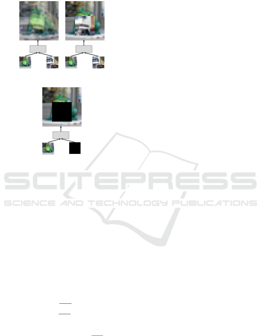
Mixup

(a)

Cutmix

(b)

Cutout

(c)

Figure 1: Visualizations of inputs and outputs of Mixup (a),

Cutmix (b), and Cutout (c) augmentation techniques.

where λ is a randomly sampled parameter from the

distribution Beta(β, β) with β being a hyperparameter.

Cutmix. Cutmix (Yun et al., 2019) relies on generat-

ing new pairs from two input pairs where a rectangu-

lar part of x

is replaced by a rectangular part of the

same size cropped from x

. It is deﬁned as



Cutmix

) = M

 x

+ (I − M

)  x

Mixup

) = λy

+ (1 − λ)y



, (3)

where M

∈ {0, 1}

W ×H

is a binary mask ﬁlled with

ones for the cropping region and zeros otherwise. I is

a binary mask ﬁlled with ones, and  is the elemen-

twise multiplication operator. The rectangle coordi-

nates deﬁned as (r

) are uniformly sampled

∼ U (0,W ), W

1 − λ = r

∼ U (0,w),

∼ U (0,H), H

1 − λ = r

∼ U (0,h), (4)

with λ being sampled from Beta(β, β) and corrected

so that the cropped area ratio becomes

×r

W ×H

= 1 − λ.

w and h denote hyperparameters.

Cutout. Cutout (DeVries and Taylor, 2017) can be

considered as a special case of Cutmix and can be ap-

plied using Eq. 3 with x

being replaced by a zero

matrix of the same dimension. However, in contrast

to Cutmix and Mixup, Cutout does not apply any op-

eration on the targets.

Visualizations of the inputs and outputs of the

Mixup with λ = 0.4, Cutmix with 1 − λ = 0.25, i.e.,

= r

= 16, and Cutout operations are shown in

Fig. 1.

RandAugment. RandAugment (Cubuk et al., 2020)

uses a set of 14 traditional augmentation transforma-

tions. Essentially, it uses two parameters, N and M,

where N is the number of augmentation transforma-

tions to apply sequentially on an image and M is the

magnitude of the different transformations.

3.2 Consistency Regularization

Augmentation methods discussed in Sec. 3.1 were ini-

tially introduced in the context of supervised learning

for enhancing the generalization capability of deep

models. Recently, ICT (Verma et al., 2019b) has

adapted interpolation consistency to semi-supervised

learning by using guessed labels of an EMA model.

The consistency term for unlabeled data becomes

= E

∈U

λ∼Beta(β,β)



(Mixup

)),Mixup

),C

))



(5)

where C

and C

refer to the classiﬁer and EMA mod-

els parameterized by θ and θ

, respectively, and l is a

measure of distance. For the supervised part, a similar

objective applies to the labeled data

= E

),(x

)∈L

λ∼Beta(β,β)



(Mixup

)),Mixup

)



. (6)

We reproduce ICT without changing any setting

using Tensorﬂow (Abadi et al., 2016). However, for

our baseline which is practically a duplicate of ICT,

we apply two changes. First, we omit the ZCA trans-

formation of the input data and only normalize the

samples to lie in the range [0,1]. Second, we rectify

a discrepancy in the target calculation in Eq. 5, i.e.,

while authors apply Mixup on the logits of C

to feed

the softmax function and calculate the targets, we ap-

ply Mixup directly on the softmax outputs. We notice

that these changes lead to a slight improvement in per-

formance.

Table 1 compares ICT to our adaptation of it,

ICT

∗

. Moreover, since our framework allows the

replacement of the Mixup operator through any in

Sec. 3.1 discussed augmentation methods, Tab. 1

shows a comparison between the three related meth-

ods Mixup, Cutmix, and Cutout on CIFAR-10 test set

using 4000 labeled samples, see Sec. 5.1. For Cut-

mix and Cutout, we use w ×h = 16 ×16 cropped area

CGT: Consistency Guided Training in Semi-Supervised Learning

Table 1: Comparison between test error rates [%] of ICT and our implementation of it (ICT

∗

) on CIFAR-10 using 4000 labels.

Errors for Cutmix, Cutout, and the two linear combinations (shown at the last two coloums) are obtained by adapting them

into ICT

∗

while replacing Mixup. Results are averaged over three runs using the CNN-13 architecture (Laine and Aila, 2016).

CIFAR-10, L = 4000

ICT Mixup (ICT

∗

) Cutmix Cutout Mixup&Cutmix Mixup&Cutmix&Cutout

7.39 ± 0.11 6.90 ± 0.16 6.73 ± 0.20 8.22 ± 0.09 6.23 ± 0.01

6.23 ± 0.01

6.23 ± 0.01 6.53 ± 0.06

size as suggested by the authors in (Yun et al., 2019;

DeVries and Taylor, 2017).

We observe that Cutmix and Mixup achieve com-

parable performances and signiﬁcantly outperform

Cutout. As discussed before, Cutout can be con-

sidered as a special case of Cutmix, however, while

Cutmix crops a region of an image and proportion-

ally adjusts the targets of the remaining patch, Cutout

omits this target adjustment. In (Yun et al., 2019), au-

thors are able to enhance the performance of Cutout

by combining it with label smoothing. Therefore, we

think that label smoothing may also help in our set-

ting. Furthermore, we observe that the two straight-

forward combinations, i.e., linear combinations of

the corresponding objectives, shown in the last two

columns, not only outperform all three basic augmen-

tation methods but Mixup&Cutmix also outperforms

more advanced and recent methods such as (Berthelot

et al., 2019; Nair et al., 2019; Ma et al., 2020), see

Tab. 2. This observation together with the simplic-

ity of those augmentation techniques motivated us to

further explore and develop this framework.

4 CGT FRAMEWORK

Our framework uniﬁes several of the previously men-

tioned augmentation techniques, namely Mixup, Cut-

mix, RandAugment, and 3-Mixup which we describe

in detail in the following section. For applying the

augmentations on unlabeled data, as for ICT, we rely

on guessed labels obtained using an EMA model, C

Moreover, we propose a procedure that slightly im-

proves the performance of ICT and its derivatives,

mentioned in the previous section, in the ﬁnal stage

of the training.

4.1 Augmentation Operators

In this section, we introduce our augmented Mixup

and Cutmix operators in addition to the 3-Mixup op-

erator which is an extension of the Mixup operator

and regularizes a larger region of the input space.

Let B = {(x

)}

i=1

≡ (X ,Y ) be a batch of B

samples, X , and their corresponding true or guessed

labels depending on whether x

∈ L or x

∈ U. We de-

note two random permutations of (X ,Y ) as (X ,Y )

and (X ,Y )

and in order to distinguish between them

elementwise, we use the following notation

(X ,Y )

≡ (X

) ≡ {(x

)}

i=1

(X ,Y )

≡ (X

) ≡ {(x

)}

i=1

. (7)

Accordingly, the following refers to the operators ap-

plied on the samples of a batch

Mixup

(X ,X

) ≡{Mixup

)}

i=1

Cutmix

(X ,X

) ≡{Cutmix

)}

i=1

. (8)

We deﬁne the following augmented Mixup and Cut-

mix operators as

Mixup

(X ,X

) ≡ {Mixup

,ζ(x

)}

i=1

, (9)

Cutmix

(X ,X

) ≡ {Cutmix

,ζ(x

)}

i=1

. (10)

Algorithm 1: Consistency Guided Training (CGT) Al-

gorithm.

Input:

epoch

, N

batch

: #epochs, #batches

B: batch size

L, U: labeled and unlabeled sets

, C

: models with parameters θ and θ

,λ

: supervised and consistency weights

w(t) ∈ [0,w

max

]: ramp-up function

τ: starting epoch for overwriting θ

β: coefﬁcient for Beta distribution

α: rate of EMA

for e = 1,...,N

epoch

for b = 1,...,N

batch

← {(x

)}

i=1

, (x

) ∈ L

← {(x

))}

i=1

, x

∈ U

λ,λ

λ = (λ

)

i=1

, λ,λ

∼ Beta(β,β)

← l

,θ,λ,λ

)

 Eq. 15

← l

,θ,λ,λ

λ,λ

)

 Eq. 18

t ← e + b/N

batch

θ ← SGD(θ,L

+ w(t)L

)

← αθ

+ (1 − α)θ

 apply EMA

end

if e ≥ τ then

θ ← θ

 overwrite θ

end

return θ

VISAPP 2022 - 17th International Conference on Computer Vision Theory and Applications





Aug



Aug



…

Aug























(a)

Mixup



(b)



Cutmix

(c)

3-Mixup

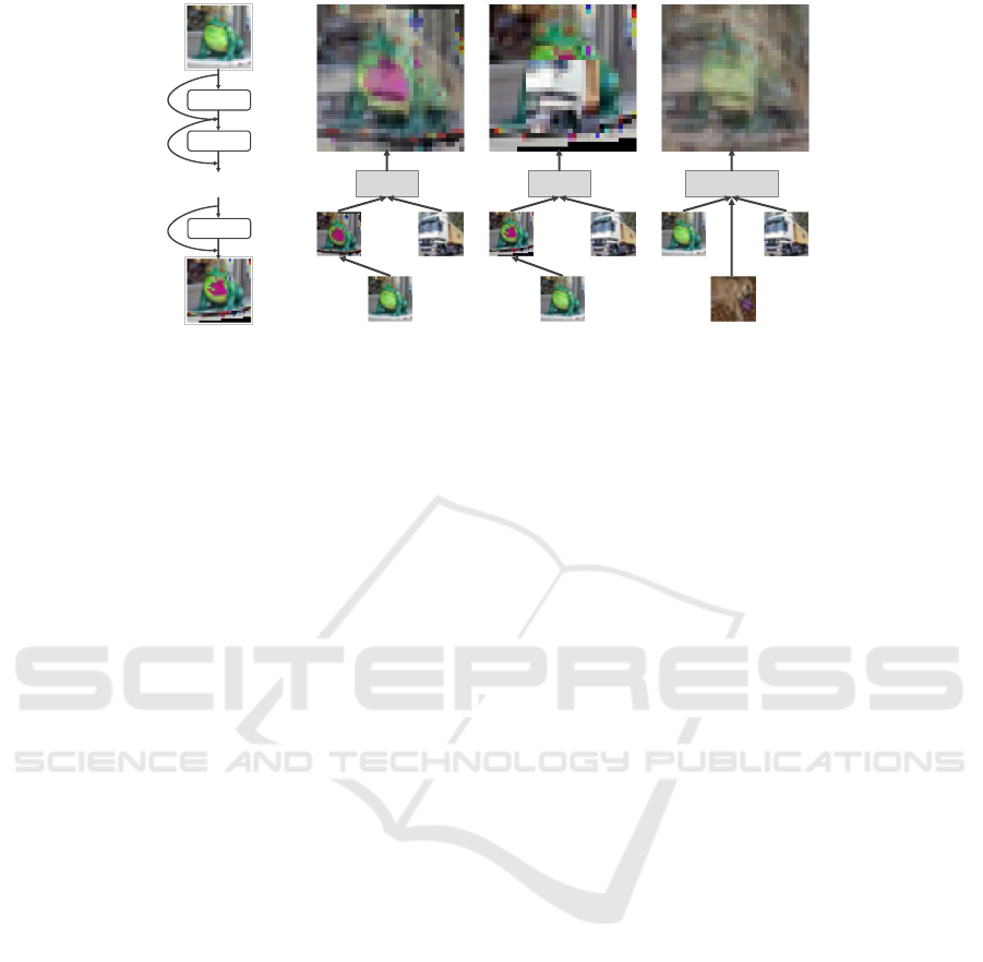
(d)

Figure 2: (a) illustrates the composite function, ζ, that applies a series of augmentation transformations stochastically with

a maximum length of d. (b) and (c) visualize our augmented Mixup and Cutmix operations, respectively. (d) visualizes the

3-Mixup operation.

The function ζ, illustrated in Fig. 2 (a), is a composite

function that applies a series of augmentation trans-

formations stochastically and has a maximum length

of d,

ζ(x, p

, p

,··· , p

) = o



···o



(x)



···



(11)

where

(x) =

(

(x) if p

< ε

x otherwise,

(12)

with o

being randomly chosen from Ω

Aug

. Ω

Aug

a set of traditional augmentation transformations, ε is

a hyperparameter, and p

is sampled from a uniform

distribution U(0,1). In Eqs. 9 and 10, we drop the

parameters of ζ for brevity. Derived from the Mixup

operator, we introduce a new operator that we name

3-Mixup and deﬁne as

3-Mixup

(X ,X

) ≡ {3-Mixup

)}

i=1

(13)

where new data pairs are created according to



3-Mixup

) =

∑

i=1

3-Mixup

) =

∑

i=1



, (14)

with λ

λ = (λ

)

i=1

and λ

being randomly sampled pa-

rameters from the distribution Beta(β,β) under the

condition

∑

i=1

= 1. The aforementioned operators

are visualized in Fig. 2.

4.2 Training Objectives

Our training routine uniﬁes the augmentation opera-

tors mentioned in Sec. 4.1. The supervised loss is

given by

(B, θ, λ,λ

) =

∑

i=1

(B, θ, λ), with (15)

(B, θ, λ) =





Mixup

(X ,X

)



,Mixup

(Y , Y

)



(16)

(B, θ, λ) =





Cutmix

(X ,X

)



,Mixup

(Y , Y

)



(17)

where CE stands for the categorical cross-entropy

function. Our consistency loss consists of three con-

tributors,

(B, θ, λ,λ

λ,λ

) =

∑

i=1

(B, θ, λ) + λ

(B, θ,λ

λ),

(18)

where l

1,2

are similar to l

1,2

except for three changes:

(a) we replace CE function with L2 function, (b) Y

are guessed labels obtained using C

(X ), and (c)

Mixup

(X ,X

) and Cutmix

(X ,X

) are replaced with

Mixup

(X ,X

) and Cutmix

(X ,X

), respectively. In

addition, we deﬁne

(B, θ,λ

λ) = L2





3-Mixup

(X ,X

)



3-Mixup

(Y , Y

)



The total loss is then calculated via Eq. 1 with

B∈L,λ

(B, θ, λ,λ

B∈U,λ,λ

(B, θ, λ,λ

λ,λ

). (19)

CGT: Consistency Guided Training in Semi-Supervised Learning

There exists a mutual inﬂuence between C

and

. In the early stages of the training, C

im-

proves rapidly and causes a slower improvement of

through EMA. However, after further training C

improves over C

and since C

functions as a target

generator, an improvement of C

leads to an improve-

ment of C

. Both models, however, reach eventually

plateaus. At that stage of the training, we notice that,

using our setting, overwriting θ with θ

periodically

starting from epoch τ leads to further improvement in

and consequently to an improvement in C

. Algo-

rithm 1 summarizes the CGT training.

5 EXPERIMENTS

5.1 Datasets

We follow the common practice in evaluating SSL

approaches (Verma et al., 2019b; Kuo et al., 2020;

Tarvainen and Valpola, 2017; Wu et al., 2019; Kam-

nitsas et al., 2018) and report the performance of

our approach on the following three SSL benchmark

datasets.

CIFAR-10. CIFAR-10 dataset (Krizhevsky, 2009)

contains colored images distributed across 10 classes.

Those classes represent objects like airplanes, frogs,

etc. It contains 50,000 training samples and 10,000

testing samples each of the size 32 × 32.

CIFAR-100. CIFAR-100 dataset (Krizhevsky, 2009)

is similar to CIFAR-10 with the same number of train-

ing and testing samples, however, it contains 100

classes.

SNHN. SVHN dataset (Netzer et al., 2011) contains

73,257 training and 26,032 testing samples. The sam-

ples are colored images of the size 32 × 32, showing

digits with various backgrounds.

For preprocessing, we normalize each sample so

that it is in the range [0,1]. For the three datasets, we

zero-pad each training sample with 2 pixels on each

side. We then crop the resulting images randomly at

the beginning of each epoch to obtain 32×32 training

samples. On CIFAR-10 and CIFAR-100, we horizon-

tally ﬂip each sample with the probability of 0.5.

For validation, we reserve 5,000 training samples

from each dataset. We train the models using a small

randomly chosen set of labeled samples (L) with re-

placement from the training set and the full training

set as unlabeled set (U) after discarding the corre-

sponding labels. We report our results on the test set

by averaging over three runs. For each dataset, we

measure the performance using different sizes of the

labeled set.

5.2 Settings

In order to emphasize the improvements driven by

our method, we use ICT settings with only two mi-

nor changes which concern the preprocessing and the

consistency regularization, see Sec. 3.2. More con-

cretely, parameters that originate from ICT settings

are learning rate, weight decay, N

epoch

, N

batch

, B, C

, w(t) ∈ [0, w

max

], β, and α. For the Cutmix oper-

ator, we use the parameters suggested in (Yun et al.,

2019), see Sec. 3.2.

Relying on the exhaustive evaluations in (Cubuk

et al., 2020), we deﬁne Ω

Aug

= {autocontrast, equal-

ize, posterize, rotate, solarize, shear-x/-y, translate-

x/-y}. For the magnitudes of the different augmen-

tation transformations, we follow (Hendrycks* et al.,

2020). Our implementation differs from RandAug-

ment (Cubuk et al., 2020) in that we randomly sam-

ple M for each operation. For the hyperparameters

of the ζ function and for τ, we conduct experiments

on the validation sets in Sec. 5.1 and ﬁnd that d = 4,

ε = 0.5, and τ = 3/4 · N

epoch

perform well across all

experiments.

We identify λ

, λ

, and w

max

as hyperparameters

to be adapted to the respective datasets. We con-

duct a search in {0,1/3,0.5} for λ

and λ

under

the conditions that

∑

= 1. For w

max

, we

search in {25, 50, 75, 100} for CIFAR-10 and SVHN.

For CIFAR-100, ICT does not provide any settings,

so in the following, we present our settings. We

notice that larger values for w

max

seem to be re-

quired on CIFAR-100, so the search space becomes

{1000,1500,2000}. Next, we give our ﬁnal settings

for the different datasets.

CIFAR-10. On CIFAR-10, for L = 4000,2000, and

1000, we use w

max

= 100, λ

= λ

= 0.5, and λ

= λ

= 1/3.

CIFAR-100. On CIFAR-100, we use N

epoch

= 900,

where we use the CIFAR-10 setting from ICT for

the ﬁrst 600 training epochs followed by 300 epochs,

where we ramp down the learning rate linearly to

a ﬁnal value of 0.0015. For L = 10000, we use

max

= 2000, λ

= λ

= 0.5, and λ

= λ

1/3. For L = 4000, we use w

max

= 1500, λ

= 1.0,

and λ

= λ

= 0.5.

SVHN. On SVHN, for L = 1000 and 500, we use

max

= 75, λ

= λ

= 0.5, and λ

= λ

= 0.5. For

L = 250, we use w

max

= 25, λ

= 1.0, and λ

= λ

0.5. In addition, following ICT, we use β = 0.1.

5.3 Results and Discussion

We report our results in terms of error rates averaged

over three runs for SVHN and CIFAR-10 test sets in

VISAPP 2022 - 17th International Conference on Computer Vision Theory and Applications

Table 2: Error rates [%] on SVHN and CIFAR-10 test sets. We ran three trials for CGT. Note that

†

refers to methods using

the WRN-28-2 architecture (Zagoruyko and Komodakis, 2016), while other methods use the CNN-13 architecture (Laine and

Aila, 2016). Both architectures are comparable in terms of size and performance as also reported in ICT (Verma et al., 2019b).

SVHN CIFAR-10

Method L = 250 L = 500 L = 1000 L = 1000 L = 2000 L = 4000

Supervised (Verma et al., 2019b) 40.62 ± 0.95 22.93 ±0.67 15.54 ± 0.61 39.95 ± 0.75 31.16 ± 0.66 21.75± 0.46

Supervised (Mixup) (Verma et al., 2019b) 33.73 ± 1.79 21.08 ±0.61 13.70 ± 0.47 36.48 ± 0.15 26.24 ± 0.46 19.67 ± 0.16

MT (Tarvainen and Valpola, 2017) 4.35 ± 0.50 4.18 ± 0.27 3.95 ± 0.19 21.55± 1.48 15.73 ± 0.31 12.31 ± 0.28

TE+SNTG (Luo et al., 2018) 5.36 ± 0.57 4.46 ± 0.26 3.98 ± 0.21 18.41± 0.52 13.64 ± 0.32 10.93 ± 0.14

MUMR

(Ghorban et al., 2021) - - 4.67 ± 0.09 - - 9.56 ± 0.23

DS (Ke et al., 2019) - - - 14.17 ± 0.38 10.72 ± 0.19 8.89 ± 0.09

ICT (Verma et al., 2019b) 4.78 ± 0.68 4.23 ± 0.15 3.89 ± 0.04 15.48± 0.78 9.26 ± 0.09 7.29 ± 0.02

AdvMixup (Ma et al., 2020) 3.95 ± 0.70 3.37 ± 0.09 3.07 ± 0.18 9.67 ± 0.08 8.04 ± 0.12 7.13 ± 0.08

RealMix

†

(Nair et al., 2019) 3.53 ± 0.38 - - - - 6.39 ± 0.27

MixMatch

†

(Berthelot et al., 2019) 3.78 ± 0.26 3.64 ± 0.46 3.27 ± 0.31 7.75 ± 0.32 7.03 ± 0.15 6.24 ± 0.06

Meta-Semi

†

(Wang et al., 2020) - 4.12 ± 0.21 3.92 ± 0.11 7.34 ± 0.22 6.58 ± 0.07 6.10 ± 0.10

AFDA

†

(Mayer et al., 2021) 3.88 ± 0.13 - 3.39 ± 0.12 9.40 ± 0.32 - 6.05 ± 0.13

PLCB (Arazo et al., 2020) 3.66 ± 0.12 3.64 ± 0.04 3.55 ± 0.08 6.85 ± 0.15 - 5.97 ± 0.15

ReMixMatch

†

(Berthelot et al., 2020) 3.10 ± 0.50 - 2.83 ± 0.30 5.73 ± 0.16

5.73 ± 0.16

5.73 ± 0.16 - 5.14 ± 0.04

FeatMatch

†

(Kuo et al., 2020) 3.34 ± 0.19 - 3.10 ± 0.06 5.76 ± 0.07 - 4.91 ± 0.18

UDA

†

(Xie et al., 2020) 5.69 ± 2.76 - 2.46 ± 0.24 - - 4.88 ± 0.18

FixMatch

†

(Sohn et al., 2020) 2.64 ± 0.64

2.64 ± 0.64

2.64 ± 0.64 - 2.36 ± 0.19

2.36 ± 0.19

2.36 ± 0.19 - - 4.31 ± 0.15

4.31 ± 0.15

CGT (ours) 2.93 ± 0.13 2.71 ± 0.07

2.71 ± 0.07

2.71 ± 0.07 2.65 ± 0.09 6.24 ± 0.27 5.61 ± 0.23

5.61 ± 0.23

5.61 ± 0.23 4.73 ± 0.09

Tab. 2 and for CIFAR-100 test set in Tab. 3.

Methods reported in Tab. 2 use either the

CNN-13 (Laine and Aila, 2016) or the WRN-28-

2 (Zagoruyko and Komodakis, 2016) architecture.

Both architectures are comparable in terms of size

and performance as also reported in ICT (Verma et al.,

2019b). For our experiments, we use the CNN-13 ar-

chitecture.

On all datasets, the test errors obtained by CGT

are competitive with other state-of-the-art SSL meth-

ods.

On SVHN, we observe that CGT results in at least

a ﬁve-fold reduction in the test error of the super-

vised learning algorithm (Verma et al., 2019b). On

SVHN and CIFAR-10, CGT performs ∼ 1 percent

point (pp) better than ICT using only one-fourth of the

maximum used labels, e.g., on CIFAR-10 using 1000

labels we achieve 6.24 ± 0.27% while ICT achieves

7.29 ± 0.02% using 4000 labels. This improvement

Table 3: Error rates [%] on CIFAR-100 test set. We ran

three trials for CGT. All methods use the CNN-13 architec-

ture (Laine and Aila, 2016).

CIFAR-100

Method L = 4000 L = 10000

MT (Tarvainen and Valpola, 2017) 45.36 ± 0.49 36.08 ± 0.51

LP (Iscen et al., 2019) 43.73 ± 0.20 35.92 ± 0.47

WA (Athiwaratkun et al., 2018) - 33.62 ± 0.54

PLCB (Arazo et al., 2020) 37.55 ± 1.09 32.15 ± 0.50

Meta-Semi (Wang et al., 2020) 37.61 ± 0.56 30.51 ± 0.32

FeatMatch (Kuo et al., 2020) 31.06 ±0.41

31.06 ± 0.41

31.06 ± 0.41 26.83 ± 0.04

CGT (ours) 31.88 ± 0.62 26.74± 0.25

26.74 ± 0.25

Table 4: Ablation study on CIFAR-10 using 4000 labeled

data points. Error rates [%] are reported across three trials.

d = i refers to applying i randomly chosen augmentation

transformations from Ω

Aug

(see 5.2) sequentially on one of

the input arguments of Mixup and/or Cutmix.

Aspect, CIFAR-10, L = 4000

Mixup Cutmix 3-Mixup d = 2 d = 4 ζ θ ← θ

Error rate [%]

X - - - - - - 6.90 ±0.16

- X - - - - - 6.73 ±0.20

X X - - - - - 6.23± 0.01

X X X - - - - 6.02 ± 0.13

X X X X - - - 5.17± 0.01

X X X - X - - 5.20 ±0.04

X X X - - X - 4.93 ± 0.11

X X X - - X X 4.73 ±0.09

is achieved through CGT’s improved loss calculation

and augmentation methods. Note that CGT’s bare-

bone, as described in Sec. 3.2 and Sec. 5.2, is ICT.

This demonstrates that CGT uses, through the intro-

duced modiﬁcations, the available labels more efﬁ-

ciently than ICT.

We observe that CGT seems to be less sensitive

to the size of the labeled set compared to our base-

line ICT. A comparison to the recent methods pre-

sented in Tab. 2 reveals that our approach is able to

achieve state-of-the-art performance on SVHN and

CIFAR-10. FixMatch (Sohn et al., 2020) which

scores slightly higher than our method requires above

1 million training steps to fully converge while our

method requires only 200 thousand training steps. In

addition, FixMatch and UDA (Xie et al., 2020) utilize

7 times more unlabeled than labeled data in each step,

which further increases the training time.

CGT: Consistency Guided Training in Semi-Supervised Learning

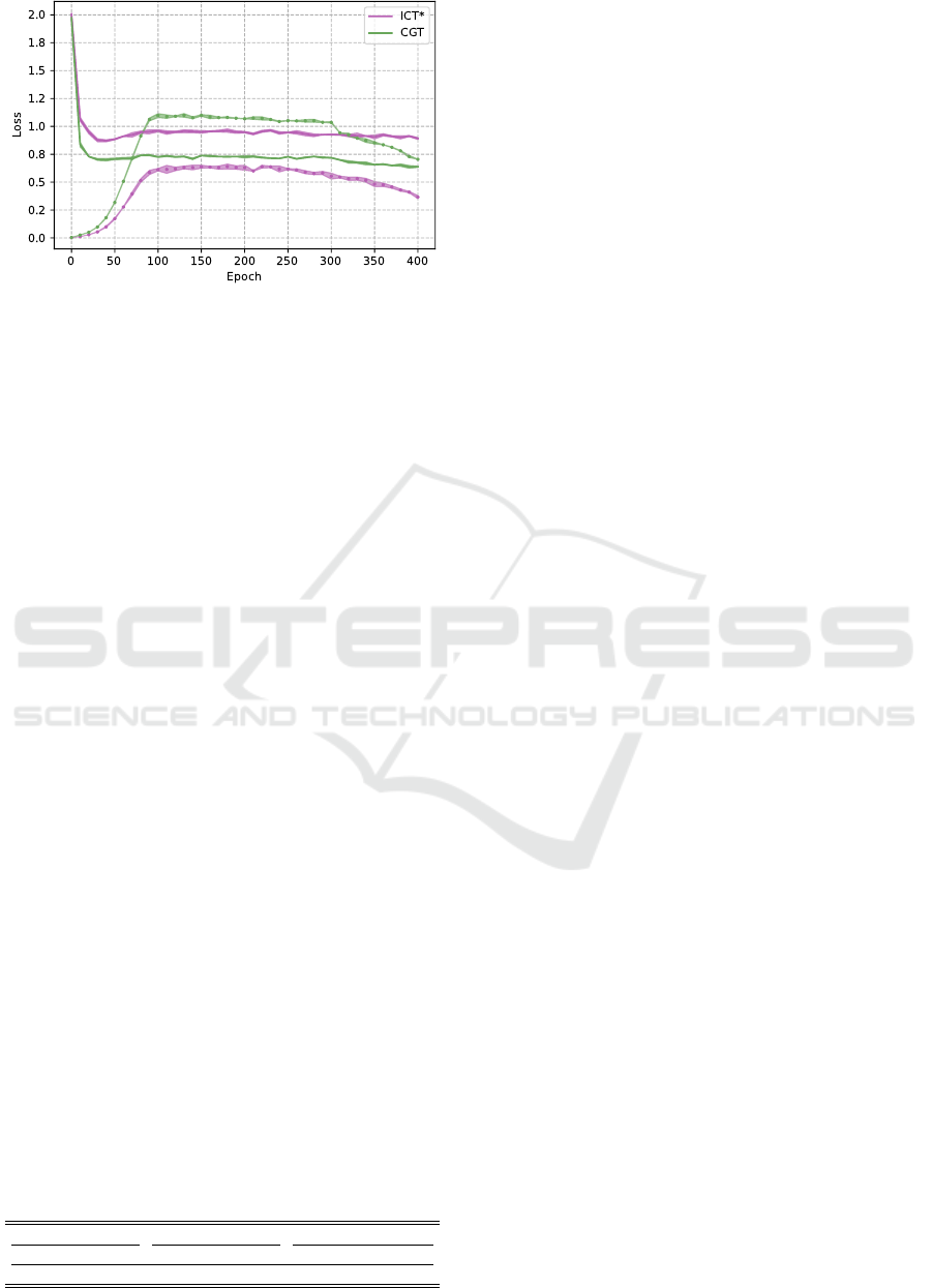
Figure 3: A comparison of the evolutions of the supervised

(solid) and consistency (dotted) losses recorded over the

training epochs for our baseline, ICT

∗

, and CGT on CIFAR-

10 using L = 4000.

Table 3 compares our results to recent methods

on CIFAR-100. Here we compare only to methods

that use the CNN-13 (Laine and Aila, 2016) archi-

tecture. Also here, we observe a competitive per-

formance of our approach when compared to recent

methods. Note that FixMatch (Sohn et al., 2020) is

not included since it reports results on CIFAR-100

using WRN-28-8 which is much larger and thus not

comparable to the above-mentioned architectures.

As described in Sec. 4, our approach in com-

posed of multiple components. In Tab. 4, we show

the contribution of each component by decomposing

our method and conducting an ablation study. We ob-

serve that applying augmentation transformations, es-

pecially through the function composite ζ has a sig-

niﬁcant contribution to the ﬁnal performance gain.

In order to determine the improvement that comes

with overwriting θ with θ

during training, we stored

each experiment from Tabs. 2 and 3 at its correspond-

ing epoch τ and continued training without overwrit-

ing θ. The achieved error rates are shown in Tab. 5.

Overwriting θ comes at virtually no additional com-

putational cost and improves the performances across

all the above experiments.

The supervised contribution to the loss function

strives to minimize the entropy of predictions while

the consistency contribution can practically lead to a

trivial solution which corresponds to a maximized en-

tropy, i.e., a zero consistency loss with θ

∗

for which

∗

) = (1/K,...,1/K) for any x

. Considering the

loss composition, the question arises: How should

Table 5: The effect of periodically overwriting θ with θ

starting from epoch τ.

SVHN CIFAR-10 CIFAR-100

L = 250 L = 1000 L = 1000 L = 4000 L = 4000 L = 10000

2.99 ± 0.10 2.69 ± 0.10 6.43 ± 0.28 4.93± 0.11 32.31 ± 0.54 27.25± 0.20

the consistency contribution behave in comparison to

the supervised one for obtaining an optimal solution

θ? Although we do not explicitly seek to answer this

question, we show in the following a related observa-

tion that we assume to be relevant for further inves-

tigation. In ICT, we notice that the supervised con-

tribution largely guides the training, i.e., it remains

higher than the consistency contribution. CGT, how-

ever, has a lower supervised contribution and a signif-

icantly higher consistency contribution. Furthermore,

the consistency contribution in CGT exceeds its su-

pervised one, see Fig. 3, seemingly without having

any negative effect on the performance.

6 CONCLUSION

In this work, we have presented a simple yet efﬁcient

SSL algorithm, Consistency Guided Training (CGT).

The CGT framework uniﬁes multiple existing image-

based augmentation techniques, namely the Mixup

and CutMix operations. In addition, it utilizes new

augmented versions of these operators where aug-

mentations are stochastically applied to one side of

the inputs of the Mixup and CutMix operators. More-

over, CGT involves a new generalization of the Mixup

operator on unlabeled samples to regularize a larger

region of the input space. The supervised and con-

sistency losses in our framework are expressed as lin-

ear combinations of multiple constituents, each corre-

sponding to a different augmentation transformation.

Furthermore, our CGT framework has demonstrated

to be beneﬁtting from heavy augmentations of the un-

labeled training data which enabled it to achieve state-

of-the-art performance on three challenging bench-

mark datasets.

REFERENCES

Abadi, M., Barham, P., Chen, J., Chen, Z., Davis, A., Dean,

J., et al. (2016). Tensorﬂow: A system for large-scale

machine learning. In Symposium on Operating Sys-

tems Design and Implementation.

Arazo, E., Ortego, D., Albert, P., O’ Connor, N. E., and

McGuinness, K. (2020). Pseudo-labeling and conﬁr-

mation bias in deep semi-supervised learning. In In-

ternational Joint Conference on Neural Networks.

Athiwaratkun, B., Finzi, M., Izmailov, P., and Wilson,

A. G. (2018). Improving consistency-based semi-

supervised learning with weight averaging. arXiv

preprint arXiv:1806.05594.

Berthelot, D., Carlini, N., Cubuk, E. D., Kurakin, A., Sohn,

K., Zhang, H., and Raffel, C. (2020). Remixmatch:

Semi-supervised learning with distribution alignment

VISAPP 2022 - 17th International Conference on Computer Vision Theory and Applications

and augmentation anchoring. In International Confer-

ence on Learning Representations.

Berthelot, D., Carlini, N., Goodfellow, I., Papernot, N.,

Oliver, A., and Raffel, C. A. (2019). Mixmatch: A

holistic approach to semi-supervised learning. In Ad-

vances in Neural Information Processing Systems.

Cubuk, E. D., Zoph, B., Mane, D., Vasudevan, V., and Le,

Q. V. (2018). Autoaugment: Learning augmentation

policies from data. arXiv preprint arXiv:1805.09501.

Cubuk, E. D., Zoph, B., Shlens, J., and Le, Q. V. (2020).

Randaugment: Practical automated data augmentation

with a reduced search space. In Proceedings of the

IEEE/CVF Conference on Computer Vision and Pat-

tern Recognition Workshops.

DeVries, T. and Taylor, G. W. (2017). Improved regular-

ization of convolutional neural networks with cutout.

arXiv preprint arXiv:1708.04552.

Ghiasi, G., Lin, T.-Y., and Le, Q. V. (2018). Dropblock: a

regularization method for convolutional networks. In

Proceedings of the International Conference on Neu-

ral Information Processing Systems.

Ghorban, F., Hasan, N., Velten, J., and Kummert, A. (2021).

Improving fm-gan through mixup manifold regular-

ization. In International Symposium on Circuits and

Systems.

Ghorban, F., Mar

ın, J., Su, Y., Colombo, A., and Kummert,

A. (2018). Aggregated channels network for real-time

pedestrian detection. In International Conference on

Machine Vision.

Goodfellow, I., Shlens, J., and Szegedy, C. (2015). Explain-

ing and harnessing adversarial examples. In Interna-

tional Conference on Learning Representations.

Hendrycks*, D., Mu*, N., Cubuk, E. D., Zoph, B., Gilmer,

J., and Lakshminarayanan, B. (2020). Augmix: A

simple method to improve robustness and uncertainty

under data shift. In International Conference on

Learning Representations.

Ho, D., Liang, E., Chen, X., Stoica, I., and Abbeel, P.

(2019). Population based augmentation: Efﬁcient

learning of augmentation policy schedules. In Inter-

national Conference on Machine Learning.

Iscen, A., Tolias, G., Avrithis, Y., and Chum, O. (2019).

Label propagation for deep semi-supervised learning.

In Proceedings of the IEEE Conference on Computer

Vision and Pattern Recognition.

Kamnitsas, K., Castro, D., Le Folgoc, L., Walker, I., Tanno,

R., Rueckert, D., Glocker, B., Criminisi, A., and Nori,

A. (2018). Semi-supervised learning via compact la-

tent space clustering. In International Conference on

Machine Learning.

Ke, Z., Wang, D., Yan, Q., Ren, J., and Lau, R. W. (2019).

Dual student: Breaking the limits of the teacher in

semi-supervised learning. In Proceedings of the IEEE

International Conference on Computer Vision.

Krizhevsky, A. (2009). Learning multiple layers of fea-

tures from tiny images. Technical report, Master’s

thesis, Department of Computer Science, University

of Toronto.

Kuo, C.-W., Ma, C.-Y., Huang, J.-B., and Kira, Z. (2020).

Featmatch: Feature-based augmentation for semi-

supervised learning. In European Conference on

Computer Vision.

Laine, S. and Aila, T. (2016). Temporal ensem-

bling for semi-supervised learning. arXiv preprint

arXiv:1610.02242.

Li, W., Wang, Z., Li, J., Polson, J., Speier, W., and Arnold,

C. W. (2019). Semi-supervised learning based on gen-

erative adversarial network: a comparison between

good gan and bad gan approach. In CVPR Workshops.

Lim, S., Kim, I., Kim, T., Kim, C., and Kim, S. (2019). Fast

autoaugment. arXiv preprint arXiv:1905.00397.

Luo, Y., Zhu, J., Li, M., Ren, Y., and Zhang, B.

(2018). Smooth neighbors on teacher graphs for semi-

supervised learning. In Proceedings of the IEEE Con-

ference on Computer Vision and Pattern Recognition.

Ma, Y., Mao, X., Chen, Y., and Li, Q. (2020). Mix-

ing up real samples and adversarial samples for semi-

supervised learning. In International Joint Conference

on Neural Networks.

Mayer, C., Paul, M., and Timofte, R. (2021). Adversar-

ial feature distribution alignment for semi-supervised

learning. Computer Vision and Image Understanding.

Miyato, T., Maeda, S.-i., Koyama, M., and Ishii, S. (2018).

Virtual adversarial training: a regularization method

for supervised and semi-supervised learning. IEEE

Transactions on Pattern Analysis and Machine Intel-

ligence.

Nair, V., Alonso, J. F., and Beltramelli, T. (2019). Realmix:

Towards realistic semi-supervised deep learning algo-

rithms. arXiv preprint arXiv:1912.08766.

Netzer, Y., Wang, T., Coates, A., Bissacco, A., Wu, B., and

Ng, A. (2011). Reading digits in natural images with

unsupervised feature learning. In Advances in Neural

Information Processing Systems.

Qiao, S., Shen, W., Zhang, Z., Wang, B., and Yuille, A.

(2018). Deep co-training for semi-supervised image

recognition. In Proceedings of the European Confer-

ence on Computer Vision.

Sohn, K., Berthelot, D., Li, C.-L., Zhang, Z., Carlini, N.,

Cubuk, E. D., Kurakin, A., Zhang, H., and Raffel, C.

(2020). Fixmatch: Simplifying semi-supervised learn-

ing with consistency and conﬁdence. arXiv preprint

arXiv:2001.07685.

Tarvainen, A. and Valpola, H. (2017). Mean teachers are

better role models: Weight-averaged consistency tar-

gets improve semi-supervised deep learning results. In

Advances in Neural Information Processing Systems.

Tokozume, Y., Ushiku, Y., and Harada, T. (2018). Between-

class learning for image classiﬁcation. In Proceedings

of the IEEE Conference on Computer Vision and Pat-

tern Recognition.

Verma, V., Lamb, A., Beckham, C., Najaﬁ, A., Mitliagkas,

I., Lopez-Paz, D., and Bengio, Y. (2019a). Manifold

mixup: Better representations by interpolating hid-

den states. In International Conference on Machine

Learning.

Verma, V., Lamb, A., Kannala, J., Bengio, Y., and Lopez-

Paz, D. (2019b). Interpolation consistency training for

semi-supervised learning. In Proceedings of the Inter-

national Joint Conference on Artiﬁcial Intelligence.

CGT: Consistency Guided Training in Semi-Supervised Learning

Wang, Y., Guo, J., Song, S., and Huang, G. (2020). Meta-

semi: A meta-learning approach for semi-supervised

learning. arXiv preprint arXiv:2007.02394.

Wu, S., Deng, G., Li, J., Li, R., Yu, Z., and Wong, H.-S.

(2019). Enhancing triplegan for semi-supervised con-

ditional instance synthesis and classiﬁcation. In Pro-

ceedings of the IEEE Conference on Computer Vision

and Pattern Recognition.

Xie, Q., Dai, Z., Hovy, E., Luong, T., and Le, Q.

(2020). Unsupervised data augmentation for consis-

tency training. Advances in Neural Information Pro-

cessing Systems.

Xie, Q., Peng, M., Huang, J., Wang, B., and Wang, H.

(2019). Discriminative regularization with conditional

generative adversarial nets for semi-supervised learn-

ing. In International Joint Conference on Neural Net-

works.

Yun, S., Han, D., Oh, S. J., Chun, S., Choe, J., and Yoo,

Y. (2019). Cutmix: Regularization strategy to train

strong classiﬁers with localizable features. In Pro-

ceedings of the IEEE/CVF International Conference

on Computer Vision.

Zagoruyko, S. and Komodakis, N. (2016). Wide residual

networks. In British Machine Vision Conference.

Zhang, H., Cisse, M., Dauphin, Y. N., and Lopez-Paz, D.

(2018). mixup: Beyond empirical risk minimization.

In International Conference on Learning Representa-

tions.

Zhong, Z., Zheng, L., Kang, G., Li, S., and Yang, Y. (2020).

Random erasing data augmentation. In Proceedings of

the AAAI Conference on Artiﬁcial Intelligence.

VISAPP 2022 - 17th International Conference on Computer Vision Theory and Applications