3-D Tennis Ball Trajectory Estimation from Multi-view Videos and Its

Parameterization by Parabola Fitting

Kenta Sohara

and Yasuyuki Sugaya

Toyohashi University of Technology, Toyohashi, Aichi, Japan

Keywords:

3-D Reconstruction, Multi-views, Parabola Fitting, Parameterization of Ball Trajectory.

Abstract:

We propose a new method for estimating 3-D trajectories of a tennis ball from multiple video sequences and

parameterizing the 3-D trajectories. We extract candidate positions of a ball by a frame difference technique

and reconstruct 3-D positions of them by two-view reconstruction for every image pairs. By analyzing a

distribution of the reconstructed 3-D points, we ﬁnd a cluster among them and decide its cluster center as the

3-D ball position. Moreover, we ﬁt a plane to the estimated 3-D trajectory and express them as a 2-D point

data. We parameterize the 2-D data by ﬁtting two parabolas to them. By simulation and real experiments, we

demonstrate the efﬁciency of our method.

1 INTRODUCTION

Recently, computer vision techniques have attracted

a lot of attention in sports analytics. For example,

in order to improve player skills, one analyzes sports

scenes by using computer vision techniques. For

judging and analyzing sports scenes, computer vi-

sion techniques are also used. In professional tennis

matches, one uses the Hawk-eye system(Hawk-Eye,

2002) to judge whether the ball bounces on the court

or not. In volleyball matches in Japan, a system that

measures a 3-D ball position and shows its trajectory

and speed is used.

We are now developing a coaching assist system

for tennis players. In this paper, we propose a new

method for estimating 3-D trajectories of a tennis ball

from multiple video sequences and parameterizing its

3-D trajectories. By using our method, we can sta-

bly compute the 3-D ball trajectory and estimate the

ball position if we cannot observe it in the input video

sequences.

Many researches for tracking a tennis ball and

players from video sequences exist. We can classify

these methods into two categories. One tracks a tennis

ball in 2-D image space. The other estimates the 3-D

ball trajectories. Yan et al. proposed a method that

tracked a tennis ball from one low quality video(Yan

et al., 2005). They extracted a ball region by a frame

https://orcid.org/0000-0003-2831-0054

https://orcid.org/0000-0002-4400-1051

difference technique and tracked it by using a particle

ﬁlter. Archana et al. detected a ball region by a frame

difference and background subtraction(Archana and

Geetha, 2015). Qazi et al. proposed a method that

extracted a ball candidate region by color information

and saliency features and decided the ball region by

the random forest method(Qazi et al., 2015). Pol-

ceanu et al. took a video by a ﬁsh-eye lens camera

and proposed a method for tracking a tennis ball in

real time(Polceanu et al., 2018). All these methods

extracted and tracked a ball in the image frames.

On the other hand, Takanohashi et al. proposed

a method for reconstructing a 3-D ball trajectory by

a shape from silhouette method(Takanohashi et al.,

2007). They also reconstructed the 3-D trajectory

from asynchronous video sequences. Fazio recon-

structed 3-D positions of the ball from two smart

phone videos. Since their method reconstructs a

ball position by two-view reconstruction, they can-

not reconstruct it if the ball is not observed in one

or both cameras. Miyata et al. proposed a method

that reconstructed a ball trajectory from multi-view

videos(Miyata et al., 2017). They automatically

synchronize video sequences from uncalibrated and

asynchronous video sequences by using an epipolar

constraint. However, they assume that a ball is ob-

served in all video sequences. In our research, we re-

construct a 3-D ball position by two-view reconstruc-

tion technique among some image pairs. Therefore,

our method can reconstruct the ball position if the ball

is not observed in some cameras.

Sohara, K. and Sugaya, Y.

3-D Tennis Ball Trajectory Estimation from Multi-view Videos and Its Parameterization by Parabola Fitting.

DOI: 10.5220/0010768700003124

In Proceedings of the 17th International Joint Conference on Computer Vision, Imaging and Computer Graphics Theory and Applications (VISIGRAPP 2022) - Volume 5: VISAPP, pages

769-776

ISBN: 978-989-758-555-5; ISSN: 2184-4321

769

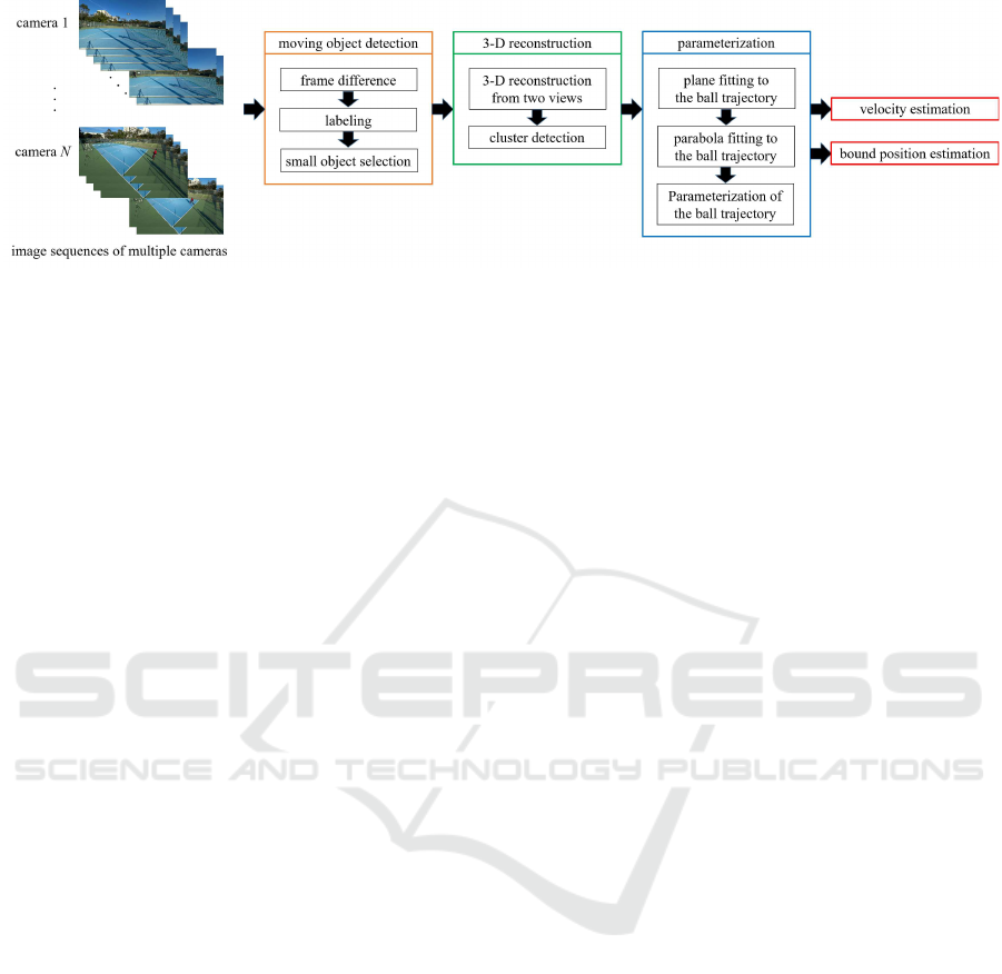
Figure 1: Illustration of our proposed method ﬂow.

2 PROPOSED METHOD

2.1 Overview of the Proposed Method

We propose a new method for estimating 3-D trajec-

tories of a tennis ball from multiple video sequences

and parameterizing them by parabola equations. By

using the parameterized trajectories, we can estimate

the ball speed and its bounced position.

We reconstruct 3-D positions of moving objects,

which are extracted by a frame difference technique,

by two-view reconstruction and decide the centroid

of a cluster points as the position of the ball. After

computing a 3-D ball trajectory, we ﬁt a plane to them

and express those trajectory as 2-D points. Then, we

ﬁt two parabolas to them and correct and interpolate

them by the ﬁtted parabola equations.

Therefore, our method has the following advan-

tages against the existing methods and these are the

contributions of this paper:

• We can obtain the 3-D ball position without decid-

ing and tracking the 2-D ball position explicitly.

This is superior to the tracking based methods.

• We can compute the ball position if we cannot ob-

serve it in some images. Miyata’s methods uses

multiple camera information, however, they as-

sume that a ball is observed in all video sequence.

• We can stably obtain the ball position compared

with a multi-view reconstruction by reducing in-

ﬂuences of miss-detection and noise of the 2-D

ball position.

• By ﬁtting a parabola to a ball trajectory, we can

estimate the 3-D ball position and its speed at an

arbitrary time.

We show the ﬂow of our proposed method in

Fig. 1. We roughly classify all the process into three

categories.

1. Ball candidate detection by a frame difference

technique

2. 3-D reconstruction of the ball trajectory

3. Parameterization of the ball trajectory

We denote the details of each process in the fol-

lowing sections.

2.2 Preprocessing

We calibrate the camera parameters and synchro-

nize all video sequences in advance. For camera

calibration, we capture a chess pattern and estimate

the intrinsic parameters of the cameras by Zhang’s

method(Zhang, 2000). Then, after ﬁxing the cameras

around the tennis court, we estimate the extrinsic pa-

rameters of the cameras, namely camera location and

pose, from the correspondences of 3-D and 2-D line

parameters of the tennis court by Zhang(Zhang et al.,

2012). For video synchronization, we manually syn-

chronize video sequences by visual inspection. The

automatic synchronization of the video sequences is a

future work.

2.3 Ball Candidate Region Extraction

For a ball region extraction from an image, we use a

well-known techniques for detecting moving objects.

We ﬁrst extract moving objects from video images by

using a frame difference technique. For a target image

(t)

at a timet, we apply pixel subtraction by I

(t−k)

and

(t+k)

and generate binary images B

(t,t−k)

and B

(t,t+k)

by thresholding, respectively. Here, k is a frame inter-

val for the frame difference.

We extract moving objects in I

(k)

by applying

AND operation for the binary images B

(t,t−k)

and

(t,t+k)

followed by morphology operation for noise

reduction. Finally, we select centroids of the detected

small objects as candidates of a tennis ball position.

Here, it is difﬁcult to select a ball among the extracted

moving objects. In this process, we do not decide one

candidate position.

VISAPP 2022 - 17th International Conference on Computer Vision Theory and Applications

770

3 3-D RECONSTRUCTION OF A

BALL TRAJECTORY

3.1 Flow of the 3-D Reconstruction

From the extracted candidate ball positions in images,

we ﬁrst make point pairs for all candidate points in all

the image frame pairs. Then, we reconstruct 3-D po-

sitions of the point pairs by two view reconstruction

method if they satisfy the epipolar constraint. We de-

tect cluster points among all the reconstructed points

and decide their centroid as a 3-D ball position.

3.2 Epipolar Constraint

For given corresponding points x

(1)

= (x

(1)

, y

(1)

, 1)

⊤

and x

(2)

= (x

(2)

, y

(2)

, 1)

⊤

between two images, the fol-

lowing epipolar equation holds:

(1)

, Fx

(2)

) = 0, (1)

where, F is a 3× 3 matrix and is called a fundamen-

tal matrix. The notation (a, b) shows an inner product

of two vectors a and b. For a point pair between two

images, we can compute the distances from a point to

the epipolar line deﬁned by the other point by chang-

ing the roll of two points. We judge that the point pair

satisﬁes the epipolar constraint if the mean distance is

small.

3.3 3-D Reconstruction from Feature

Points

If we know the matrix A

(k)

deﬁned from the k-th

camera intrinsic parameters and the camera motion

(k)

, t

(k)

}, we can reconstruct a 3-D point from

N(N ≥ 2) correspondences of image points(Hartley

and Zisserman, 2004; Kanatani et al., 2016).

In our method, we only detect moving objects in

an image space, namely a ball position are identiﬁed.

Therefore, we ﬁrst reconstructa 3-D point from all the

detected point pairs if they satisfy the epipolar con-

straint.

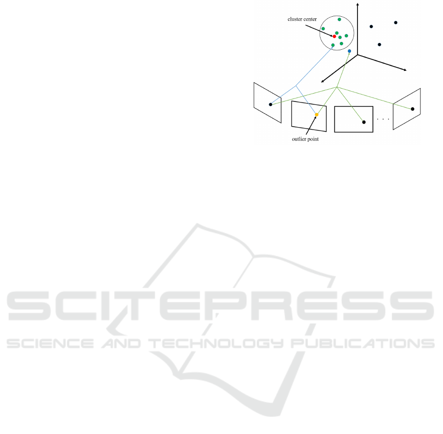
3.4 Decision of the 3-D Ball Position

After reconstructing 3-D points by two-view recon-

struction, we detect a cluster among them. For each 3-

D point, we count neighboring points whose distance

from the target point are smaller than a pre-deﬁned

threshold and we regard the point whose neighbor-

ing points are maximum and its neighboring points

as the cluster points. By considering the consis-

tency between consecutive frames, we detect a cluster

Figure 2: 3-D reconstruction of multi-view reconstruction

and cluster center.

which exists near the detected clusters in neighboring

frames. Then, we decide the centroid of those cluster

points as a 3-D ball position.

This 3-D position is not a reconstructed point from

image feature points, however, we consider that the

centroid of the cluster points is similar to a point re-

constructed by a multi-view reconstruction, because

the multi-view reconstruction computes the point so

as to minimize the sum of the distances from the lines

of view points passing through the feature points. So,

we think that if we have no outlier image points,

the accuracy of the 3-D points reconstructed from

the multi-view reconstruction and the cluster center

are almost same. However, if we have outliers from

which the reconstructed 3-D points are in the cluster(a

yellow point in Fig. 2), the accuracy of 3-D point re-

constructed by a multi-view construction may deteri-

orate(a blue point in Fig. 2).

Therefore, our method has the advantage that we

can stably obtain the ball position compared with a

multi-view reconstruction by reducing inﬂuences of

miss-detection and noise of the 2-D ball position. We

conﬁrmed this advantage in the experiment section.

4 PARAMETERIZATION OF

BALL TRAJECTORY

For parameterizing the computed ball trajectory, we

apply the following processes:

1. In order to express the 3-D trajectory points as a

2-D point sequence, we ﬁt a plane to them and

project them onto the ﬁtted plane.

2. We ﬁt two parabolas to the 2-D point sequence

and express it by parabola equations.

Since a ball trajectory is not a strict parabola

shape, we divide the computed trajectory into two

3-D Tennis Ball Trajectory Estimation from Multi-view Videos and Its Parameterization by Parabola Fitting

771

partial data with overlap and ﬁt two parabolas to

them, respectively.

3. We correct the observed points and interpolate the

missing points by the computed parabola equa-

tions.

By parameterizing the ball position for parabola

equations, we can estimate a bounce position of the

ball if we cannot observe it in images.

4.1 Plane Fitting to the 3-D Trajectory

In order to express a 3-D trajectory of a ball as a 2-D

data, we ﬁrst ﬁt a plane to the 3-D trajectory. A plane

equation in 3-D space can be written in the form

Ax+ By+Cz+ D = 0. (2)

For 3-D trajectory r

= (x

, y

, z

)

⊤

, α = 1, ..., N, if

we deﬁne a data vector ξ

= (x

, y

, z

, 1)

⊤

and a pa-

rameter vector u = (A, B, C, D)

⊤

, we have (ξ

, u) ≈ 0

in the presence of the noise.

The simplest method for computing the plane pa-

rameter u is the least squares and the solution is given

by minimizing the following function:

J =

∑

α=1

(ξ

, u)

= (u, Mu), M =

∑

α=1

⊤

(3)

As we know, the solution of the least squares is given

as the unit eigenvector of the smallest eigenvalue of

the matrix M. In this paper, by considering the pres-

ence of outlier points, we ﬁt a plane in the RANSAC

mechanism(Fischler and Bolles, 1981). After com-

puting a plane parameter vector u, we compute a pro-

jection matrix P by

P = I − nn

⊤

, n = N[(A, B, C)

⊤

], (4)

where, I is a 3× 3 identity matrix and N[a] is a nor-

malization operator that normalizes a vector norm to

be 1.

Them, we compute the 3-D data r

′

by projecting

the 3-D data r

onto the plane that is parallel to the

ﬁtted plane and passes through the origin as follows:

′

= Pr. (5)

4.2 Rotation of the Plane

Since we parameterize a ball motion in 2-D space, we

need to restore the estimated ball position to a 3-D

data. Therefore, we rotate the ﬁtted plane so that the

rotated plane is parallel to the YZ plane in the world

coordinate system and express the trajectory data as

2-D data in this plane. By this way, we can obtain

a 3-D ball position at an arbitrary time by applying

inverse rotation for the estimated 2-D position.

For computing such a rotation, we consider a ro-

tation such that the normal vector of the ﬁtted plane

and the two vectors that span the plane correspond to

the XYZ axes of the world coordinate system.

By applying this rotation to the projected trajec-

tory points, we have the 3-D data whose X values are

0. We select Y and Z values of the 3-D data and ex-

press it as 2-D data. Then we use it for a parabola

ﬁtting.

4.3 Parabola Fitting to the 2-D

Trajectory

In our method, we assume the following parabola

equation without rotation.

+ 2Bx+ 2Cy+ D= 0. (6)

We deﬁne a data vector ξ and a parameter vector u in

ξ =













, u =













, (7)

Eq. (6) is written by (ξ, u) = 0. Therefore, we can

compute the parabola parameter u by the same way

of the plane ﬁtting. Moreover, we also apply the

RANSAC to a parabola ﬁtting by considering the

presence of outlier points.

4.4 Correction and Interpolation of

Data

Based on the ﬁtted parabola, we project the observed

data onto it and interpolate the missing data, for ex-

ample, removed points as outliers of a plane and a

parabola ﬁtting.

In order to project a 2-D point onto the ﬁtted

parabola, we need to compute the its foot of the

perpendicular line. However, since it is difﬁcult

to compute it analytically, we apply the Sugaya’s

method(Sugaya, 2010) to the parabola equation de-

ﬁned by Eq. (6). For limitation of the paper space, we

omit the details of the algorithm.

We interpolate the missing points linearly by using

the corrected points and the ﬁtted parabola equation.

5 EXPERIMENTAL RESULTS

5.1 Simulation for Quantitative

Evaluation

We ﬁrst evaluated the accuracy of the 3-D reconstruc-

tion by simulated data. We virtually ﬁxed 16 cameras

VISAPP 2022 - 17th International Conference on Computer Vision Theory and Applications

772

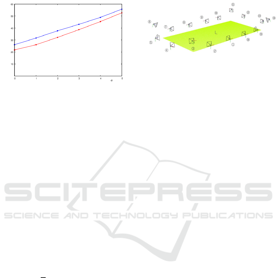
Figure 3: Comparison of 3-D reconstruction error. the blue

line: multi-view reconstruction, the red line: the proposed

method.

around a tennis court. Their positions are almost same

as shown in Fig. 4. We deﬁned the origin of a world

coordinate system at the center of the tennis court

and set X, Y, and Z axes as red , green and blue line

shown in the Fig. 4, respectively. We randomly gener-

ated 10000 points in the tennis court space with 3000

mm height, namely, −5485 ≤ x ≤ 5485, −11885 ≤

y ≤ 11885, and 0 ≤ z ≤ 3000, in millimeter unit, re-

spectively, and projected them onto the virtual im-

age planes with 1920 × 1080 pixels. If the projected

points were out of the image frame, we judged that we

could not observe the ball from these cameras. Then,

we added independent Gaussian noise of mean 0 and

standard deviation σ, σ = 0.0, 1.0, ..., 5.0 to the x and

y coordinates of the projected image points. For real-

izing outlier points, we randomly selected from 0 to 5

cameras and add independent Gaussian noise of mean

5.0+2σ and standard deviation σ, σ = 0.0, 1.0, ..., 5.0

to its projected points. Then, we estimated their 3-D

positions by the proposed method and a multi-view

reconstruction.

Figure 3 shows the average error computed by

∑

α=1

(α)

− X

(α)

k, (8)

where

(α)

and X

(α)

are the true position and the esti-

mated 3-D position of the α-th point, respectively and

N is the number of points. The horizontal axis shows

the standard deviation σ for Gaussian noise. In this

experiment, we set the threshold for ﬁnding a cluster

points to be 200 [mm]. From the result of Fig. 3, the

proposed method is superior to the multi-view recon-

struction.

5.2 Conditions of Real Experiments

We ﬁxed 16 cameras around a tennis court and cap-

tured tennis scenes by the SONY FDR-X3000 at 120

Figure 4: Calibrated camera positions.

fps. The image size is 1920 × 1080 pixels. We man-

ually calibrated camera extrinsic parameters by 2-D

and 3-D line correspondences. Figure 4 showsthe cal-

ibrated camera positions. We manually synchronized

all video sequences and tested our method for the

eleven divided partial sequences. We set the thresh-

old for ﬁnding a cluster points to be 200 [mm]. For

RANSAC, we stop iteration if the solution does not

change 200 times consecutively.

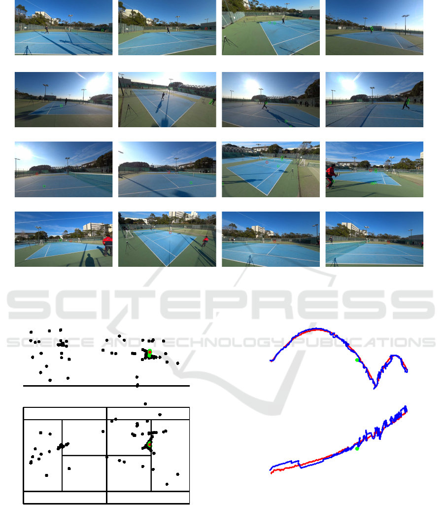
5.3 Reconstructed 3-D Ball Trajectories

Figure 5 shows ball candidate points detected by a

frame difference. For these candidate points, we made

stereo pairs and reconstructed 3-D positions of them

if the stereo pairs satisfy the epipolar constraint. The

green and red circles in Fig. 5 show the detected can-

didate points. From Fig. 5, we can see that the mov-

ing objects which are not a tennis ball, for example

human and its shadow, are also detected. Figure 6

shows the reconstructed 3-D points of the detected

moving objects in the 2925-th frame, which is in the

6-th partial sequence. The black points are all the re-

constructed points and the green points indicate the

selected cluster points, and the red is their centriod.

The red circle in Fig. 5 shows the position used by

two-view reconstruction of the green cluster points.

We also show the 3-D trajectory of the 6-th partial

sequence in Fig. 7. The red line shows the result of

our method and the blue line shows the results of a

multi-view reconstruction. We used the cluster point,

which are the green pointsin Fig. 6, for the multi-view

reconstruction. As you can see, our method gives sta-

ble results compared with the multi-view reconstruc-

tion. The green point is the 3-D point of the 2925-th

frame reconstructed by the multi-view reconstruction.

By checking the ball position of the 14-th camera in

Fig. 5, we ﬁnd that the detected ball position is not a

correct ball position. From this result, we conﬁrmed

the our method could reduce the inﬂuence of such a

miss detection and obtain a stable result.

We show the reconstructed ball trajectories of all

sequences in Fig. 8.

3-D Tennis Ball Trajectory Estimation from Multi-view Videos and Its Parameterization by Parabola Fitting

773

Camera 1 Camera 2 Camera 3 Camera 4

Camera 5 Camera 6 Camera 7 Camera 8

Camera 9 Camera 10 Camera 11 Camera 12

Camera 13 Camera 14 Camera 15 Camera 16

Figure 5: Detected ball candidate points. The center of green circle, including a red circle, indicates a candidate of the ball

position extracted by a frame difference. Red circle indicates the ball position used by two-view reconstruction of selected

cluster points.

(a) Side view

(b) Top view

Figure 6: 3-D reconstruction of the ball candidate points.

Green points indicate cluster points. Red point indicates

centroid of the cluster. Black points indicate the others.

5.4 Results of Ball Trajectory

Parameterization

For the computed 3-D trajectories, we manually

selected partial trajectories which lie on the ﬁrst

(a) Side view

(b) Top view

Figure 7: Computed 3-D trajectory. Red line indicates the

result of our method. Blue line is the result of a multi-

view reconstruction. Green point is the 3-D point of 2925-th

frame reconstructed by the multi-view reconstruction.

parabola shape and parameterized them as parabola

equations.

We ﬁtted a plane to the estimated 3-D ball trajec-

tory and expressed it as a 2-D point sequence. Next,

we ﬁtted two parabolas to the 2-D points and cor-

rected and interpolated them by the ﬁtted parabolas.

VISAPP 2022 - 17th International Conference on Computer Vision Theory and Applications

774

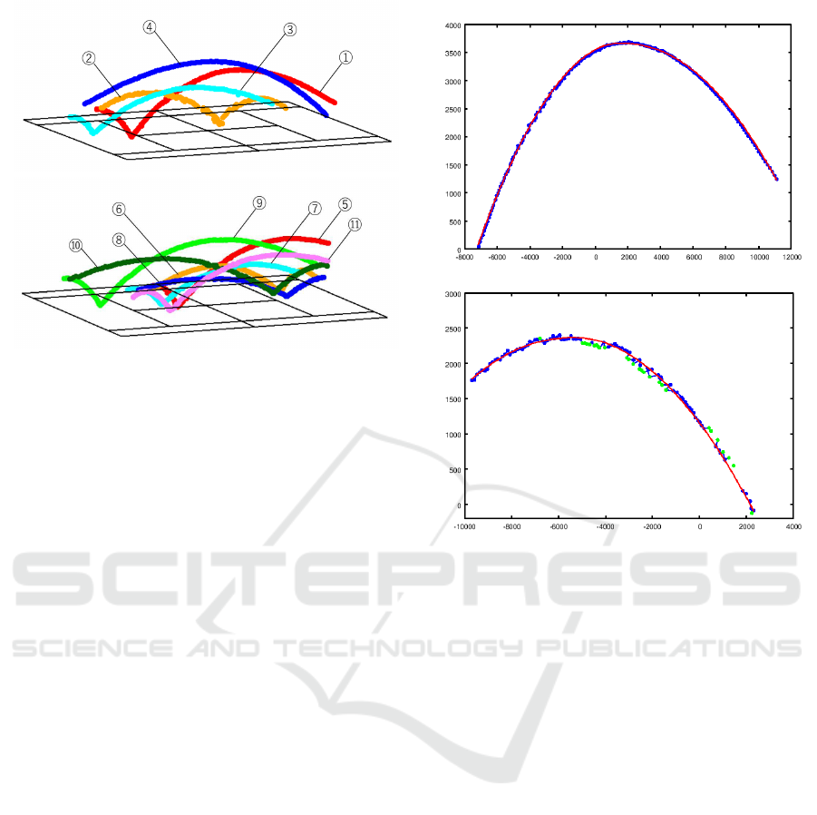
Figure 8: Reconstructed ball trajectories.

Figure 9 shows the results for the two trajectories (1)

and (2) in Fig. 8. The blue points show the input 2-D

points computed by a plane ﬁtting and the red points

are the result of data correction and interpolation.

Since the input data of Fig. 9(a) is accurately es-

timated data, outlier points are not detected on the

plane ﬁtting and the parabola ﬁtting processes and the

result of our method matches to the input data very

well. On the other hand, the input data of Fig. 9(b)

is very noisy and there exists outlier points. The

green points in Fig. 9(b) are the outlier points de-

tected by the parabola ﬁtting. However, the result of

our method is very smooth and matches to the input

data.

5.5 Estimation of Unobserved Ball

Position

Finally, we estimated a bounce position of the ball

of the trajectory data (4) in Fig. 8. The last image

frame of this sequence corresponds to an immediately

before frame that the ball bounces.

Figure 10(a) shows the result of bounce position

estimation. The blue points are the observed ball po-

sitions in a 2-D space and the red line is the ﬁtted

parabola to the latter data of the observed points. The

black line corresponds the ground of the world coor-

dinate system. We computed the intersection between

the parabola and the ground line. The green point

shows the computed intersection. We restored this

intersection to the 3-D point in the world coordinate

system and obtained the coordinates as (-1173.88,

11912.33, 0). Since the length from the court center

to the end line is 11885[mm] in deﬁnition and we as-

sume the radius of the ball is 33.5[mm], we will judge

that the ball bounces on the court.

(a) trajectory data of Fig. 8 (1)

(b) trajectory data of Fig. 8 (2)

Figure 9: 2-D ball trajectory. Blue points are the computed

2-D ball trajectory obtained from 3-D trajectory. Red points

are the corrected and interpolated points by our parabola

ﬁtting method.

Figures 10(b) and (c) show the ball positions in the

last frame of this trajectory data. We can see that the

ball is located near the end line and we do not judge

whether the ball bounces in the court or not. The red

points are the computed 2-D image position from the

estimated 3-D ball positions and the blue point shows

the estimated bounce position.

We also estimated un-reconstructed ball positions.

Since we set a frame difference parameter k be 2, we

could not estimate 3-D positions of the ball in the last

two frames. So, we estimated their positions by inter-

polating them based on the ﬁtted parabola equation.

The green points in Figs. 10(b) and (c) show their es-

timated positions. As we can see that the last green

point is drawn on the ball.

6 CONCLUSIONS

We proposed a new method for estimating 3-D trajec-

tories of a tennis ball from multiple video sequences

and parameterizing the 3-D trajectories by parabola

equations. We reconstructed 3-D ball positions of the

3-D Tennis Ball Trajectory Estimation from Multi-view Videos and Its Parameterization by Parabola Fitting

775

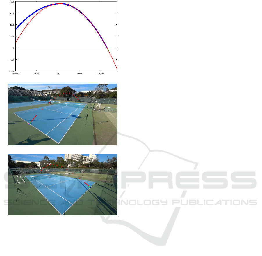
(a) Bounce position estimation in 2-D space.

(b) View from the camera No. 11 in Fig. 4

Figure 10: Bounce position estimation result for the trajec-

tory data of Fig. 8 (4).

extracted candidate 2-D position by two-view recon-

struction for every image pairs. By analyzing a distri-

bution of the reconstructed 3-D points, we decided a

centroid of the cluster as the 3-D ball position. More-

over, we parameterized the 3-D ball trajectories by

ﬁtting two parabolas to them.

In our simulation and real video experiments, we

conﬁrmed that our method stably estimated the 3-

D ball trajectory compared with a multi-view recon-

struction method. We also conﬁrmed that a ball tra-

jectory can be accurately parameterized by simple

parabola equations. We also estimated a bounce posi-

tion by using our parameterization result.

In future works, we plan to tackle automated syn-

chronization of input video sequences by using an

epipolar constraint. We also plan that we measure a

ball speed by a speed gun and compare it with the

speed estimated from our 3-D reconstruction results.

REFERENCES

Archana, M. and Geetha, M. K. (2015). Object detec-

tion and tracking based trajectory in broadcast tennis

video. Procedia Computer Science, 58:225–232.

Fischler, M. A. and Bolles, R. C. (1981). Random sample

consensus: A paradigm for model ﬁtting with applica-

tions to image analysis and automated cartography. In

Communications of the ACM, volume 24, pages 381–

395.

Hartley, R. and Zisserman, A. (2004). Multiple View Geom-

etry in computer vision. Cambridge University Press.

Hawk-Eye (2002). http://www.hawkeyeinnnovations.co.uk.

Kanatani, K., Sugaya, Y., and Kanazawa, Y. (2016). Guide

to 3D Vision Computation: Geometric Analysis and

Implementation. Stringier International.

Miyata, S., Saito, H., Takahashi, K., Mikami, D., Isogawa,

M., and Kimata, H. (2017). Ball 3d trajectory recon-

struction without preliminary temporal and geometri-

cal camera calibration. In IEEE Conference on Com-

puter Vision and Pattern Recognition Workshop, pages

164–169.

Polceanu, M., Petac, A. O., Lebsir, H. B., Fiter, B., and

Buche, C. (2018). Real time tennis match tracking

with low cost equipment. In The Thirty-First Interna-

tional Florida Artiﬁcial Intelligence Research Society

Conference(FLAIRS-31), pages 197–200.

Qazi, T., Mukherjee, P., Srivastava, S., Lall, B., and

Chauhan, N. R. (2015). Automated ball tracking in

tennis videos. In Third International Conference on

Image Information Processing, pages 236–240.

Sugaya, Y. (2010). Ellipse detection by combining division

and model selection based integration of edge points.

In Proceedings of the 4th Paciﬁc-Rim Symposium on

Image and Video Technology, pages 64–69.

Takanohashi, K., Manabe, Y., Yasumuro, Y., Imura, M., ,

and Chihara, K. (2007). Measurement of 3d ball tra-

jectory using motion blur. IPSJ Transactions of Com-

puter Vision nad Image Media, 48(SIG 1):35–47.

Yan, F., Christman, W., and Kittler, J. (2005). A tennis ball

tracking algorithm for automatic annotation of tennis

match. In British Machine Vision Conference 2005.

Zhang, X., Sun, X., Yuan, Y., Zhu, Z., and Yu, Q. (2012).

Iterative determination of camera pose from line fea-

tures. In International Archives of the Photogramme-

try, Remote Sensing and Spatial Information Sciences,

volume XXXIX-B1, pages 81–86.

Zhang, Z. (2000). A ﬂexible new technique for camera cal-

ibration. IEEE Transactions on Pattern Analysis and

Machine Intelligence, 22(11):1330–1334.

VISAPP 2022 - 17th International Conference on Computer Vision Theory and Applications

776