Forecasting Thresholds Alarms in Medical Patient Monitors using Time

Series Models

Jonas Chromik

1 a

, Bjarne Pﬁtzner

1 b

, Nina Ihde

1 c

, Marius Michaelis

1 d

, Denise Schmidt

1 e

Sophie Anne Ines Klopfenstein

2 f

, Akira-Sebastian Poncette

2 g

, Felix Balzer

2 h

and Bert Arnrich

1 i

Hasso Plattner Institute, University of Potsdam, Germany

Charité – Universitätsmedizin Berlin, Berlin, Germany

Keywords:

Patient Monitor Alarm, Medical Alarm, Intensive Care Unit, Vital Parameter, Time Series Forecasting, Alarm

Forecasting, Alarm Fatigue.

Abstract:

Too many alarms are a persistent problem in today’s intensive care medicine leading to alarm desensitisation

and alarm fatigue. This puts patients and staff at risk. We propose a forecasting strategy for threshold alarms

in patient monitors in order to replace alarms that are actionable right now with scheduled tasks in an attempt

to remove the urgency from the situation. Therefore, we employ both statistical and machine learning mod-

els for time series forecasting and apply these models to vital parameter data such as blood pressure, heart

rate, and oxygen saturation. The results are promising, although impaired by low and non-constant sampling

frequencies of the time series data in use. The combination of a GRU model with medium-resampled data

shows the best performance for most types of alarms. However, higher time resolution and constant sampling

frequencies are needed in order to meaningfully evaluate our approach.

1 INTRODUCTION

Alarm fatigue is a persisting problem in today’s in-

tensive care medicine with negative outcomes for pa-

tients and staff (Cvach, 2012). Although the problem

is well understood from a medical point of view, there

is no sufﬁcient technical solution to the alarm fatigue

yet. Among the alarms produced by medical patient

monitors, threshold alarms are of particular interest.

Alarms, in general, are supposed to express acute crit-

ical events that need immediate attention. This is, for

example, the case with arrhythmia alarms. Thresh-

old alarms, however, do not necessarily result from

https://orcid.org/0000-0002-5709-4381

https://orcid.org/0000-0001-7824-8872

https://orcid.org/0000-0001-5776-3322

https://orcid.org/0000-0002-6437-7152

https://orcid.org/0000-0002-6299-0738

https://orcid.org/0000-0002-8470-2258

https://orcid.org/0000-0003-4627-7016

https://orcid.org/0000-0003-1575-2056

https://orcid.org/0000-0001-8380-7667

an acute event but can be the result of a continued

trend as we learned from a contextual inquiry at an

intensive care unit (ICU).

In this paper, we want to forecast the foreseeable

share of threshold alarms in order to transform these

alarms into scheduled tasks, thus removing the ur-

gency of the situation. Rather than having an alarm

that has to be taken care of immediately, we want to

present scheduled tasks to the medical staff. For ex-

ample: "In approximately one hour the blood pressure

of the patient will rise above the high threshold. Dur-

ing the next hour, some member of staff should take

care of this issue." This is especially relevant since the

majority of audible and actionable alarms are thresh-

old alarms (Drew et al., 2014).

Forecasting threshold alarms is done in this work

by means of time series models, such as autoregres-

sive integrated moving average (ARIMA) models and

recurrent neural networks (RNNs). As data source we

chose the MIMIC-III database (Johnson et al., 2016)

since this is – to the best of our knowledge – the only

clinical database containing data on patient monitor

alarms. Our approach is optimised for high speci-

Chromik, J., Pﬁtzner, B., Ihde, N., Michaelis, M., Schmidt, D., Klopfenstein, S., Poncette, A., Balzer, F. and Arnrich, B.

Forecasting Thresholds Alarms in Medical Patient Monitors using Time Series Models.

DOI: 10.5220/0010767300003123

In Proceedings of the 15th International Joint Conference on Biomedical Engineering Systems and Technologies (BIOSTEC 2022) - Volume 5: HEALTHINF, pages 26-34

ISBN: 978-989-758-552-4; ISSN: 2184-4305

ﬁcity rather than high sensitivity since we acknowl-

edge that not all threshold alarms are the continuation

of a prolonged trend and hence foreseeable. We want

to avoid exacerbating the problem of alarm fatigue by

false positives of our approach.

The rest of this work is structured as follows: In

section 2 we describe the data and models we use

in this work. In section 3 we present the results we

achieve with our approach. In section 4 we discuss

these results. Finally, in section 5 we conclude our

work.

2 MATERIALS & METHODS

In order to forecast threshold alarms in medical pa-

tient monitors, we need both data on said threshold

alarms and means to forecast the corresponding vi-

tal parameter. As data source, we use the MIMIC-III

clinical database as we describe in section 2.1. As

forecasting methods, we compare a variety of time se-

ries models as we describe in section 2.2.

2.1 Materials

The MIMIC-III database contains 26 tables provid-

ing a wide range of information on the events at the

ICUs of Beth Israel Deaconess Medical Center. For

our use case, however, only the CHARTEVENTS ta-

ble is of interest. This table contains, among others,

measured values and alarm thresholds of a variety of

vital parameters such as heart rate (HR), respiratory

minute volume (MV), non-invasively measured sys-

tolic blood pressure (NBP

), respiratory rate (RR),

and peripheral blood oxygen saturation (SpO

). For

forecasting, we require time series with sufﬁciently

high and relatively stable sampling frequencies over

an extended period of time. This is not the case for

all vital parameters. Thus, we chose to use only HR,

NBP

, and SpO

as these vital parameters satisfy the

aforementioned requirements. Speciﬁcally, we are in-

terested in the data items listed in table 1.

2.2 Methods

We want to apply time series forecasting on the vi-

tal parameter data described in section 2.1 in order

to achieve our ultimate goal of forecasting threshold

alarm events. To do this, we require methods for fore-

casting time series. For this work, we decided to em-

ploy two fundamental approaches: statistical models

and machine learning models.

Statistical models aim at forecasting the future of

a time series with only the time series itself as prior

Table 1: Complete list of ITEMIDs in the CHARTEVENTS

table that are relevant for this work.

ITEMID Label

220045 HR

220046 HR Alarm - High

220047 HR Alarm - Low

220179 NBP

223751 NBP

Alarm - High

223752 NBP

Alarm - Low

220277 SpO

223769 SpO

Alarm - High

223770 SpO

Alarm - Low

knowledge. Speciﬁcally, we are using the ARIMA

model and its variation additionally featuring exoge-

nous variables (ARIMAX).

Machine learning (ML) models learn from train-

ing data and can then be applied to previously unseen

test data. In our case, we employ RNNs trained with

80% of the available vital parameter time series to

forecast on the remaining 20% of vital parameter time

series. Speciﬁcally, we are using vanilla RNNs, gated

recurrent units (GRUs), and long short-term memory

neural networks (LSTMs) because variations of recur-

rent neural networks is what is usually used on time-

series data, e.g. in (Mussumeci and Coelho, 2020),

(Pathan et al., 2020), and (Dai et al., 2021).

We frame the problem as a regression problem,

i.e. forecasting the vital parameter, instead of a clas-

siﬁcation problem, i.e. predicting whether an alarm

will occur or not, because we want to keep the ML

approach as close to the ARIMA approach as possi-

ble to ensure comparability. For the same reason, we

also do not provide additional information such as age

or sex to the ML models.

Resampling and Chunking. Both statistical and

machine learning models have in common that they

require constant sampling frequencies which are not

always given in medical databases. We address this

issue by resampling the vital parameter measurement

from the MIMIC-III database to one sample per hour

( f

= 1 h

−1

) which is close to the database’s original

sampling frequency present in most cases.

For resampling, we employ three different strate-

gies in order to fuse samples together: Minimum re-

sampling, maximum resampling, and median resam-

pling. Thus, we create three distinct but related time

series which can be used for forecasting.

Furthermore, we use a chunking strategy. We no-

ticed that there are gaps in the time series, i.e. ex-

tended periods of time where there are no data points.

We assume, that this is due to the patient being in

a different ward, surgery, or some other procedure.

Forecasting Thresholds Alarms in Medical Patient Monitors using Time Series Models

These missing data pose a difﬁculty for resampling.

Hence, we subdivide the data of a patient’s ICU stay

along the data gaps into multiple chunks and operate

only on these chunks throughout the rest of our work.

By subdividing the patients’ data into chunks and

treating these chunks as distinct time series, we cir-

cumvent a missing data issue. In practice, this im-

plies that whenever a period of missing data arises, the

model has to re-learn and cannot build upon the data

from the prior chunk. Nevertheless, we reason that

this approach makes sense because we cannot know

what happened in the period of missing data. For ex-

ample, when the period of missing data was caused by

a surgical procedure, the patient might be in a com-

pletely different condition after the surgery than be-

fore. Consequently having a completely different vi-

tal parameter distribution that can not be associated

with the period before the surgery.

Experiment Setup. Regardless of whether the

model in use is a statistical model or a ML model,

we always employ the same experiment setup: We

use 12 or 30 timesteps (lags) equivalent to 12 or 30

hours of vital parameter data as input for the model.

We chose these speciﬁc periods because we wanted to

compare performances for a rather short and a rather

long observation. The 12 hours period primarily aims

at providing clinicians with alarm forecasts in a timely

manner. With this approach, forecasts are provided

after the patient spent half a day at the ICU. In con-

trast, the 30 hours time frame aims at sufﬁciently

spanning a complete cycle of the circadian rhythm

hence giving a more holistic picture of the patient’s

vital parameter distribution.

The model produces a forecasted value for the

hour following the input lags. We compare the fore-

casted value to the currently active high or low alarm

threshold. If the value is above the high threshold or

below the low threshold, a respective threshold alarm

is forecasted. Otherwise, no alarm is forecasted. Sub-

sequently, we compare the forecast with the actual

situation, i.e. whether there was actually a threshold

alarm triggered by the actual vital parameter measure-

ment.

This common approach is used for all models

we evaluated. However, details differ since there

are conceptual differences between the models. The

most striking one is that ML models require dedicated

training data while statistical models learn only on the

given input sequence. Hence, we describe the con-

crete experiment setups for speciﬁc models in the fol-

lowing.

Statistical Models. We use both ARIMA and ARI-

MAX models as can be seen in Table 2. The ARIMA

models are used with the median and minimum or

maximum resampled time series. For ARIMAX we

use the maximum resampled time series for fore-

casting high threshold alarms and the minimum re-

sampled time series for forecasting the low threshold

alarms. For both ARIMAX cases, the median resam-

pled time series is used as exogenous series. All three

described model setups are processed with a train size

of 12 lags or 30 lags, respectively, which determines

the minimum length of chunks required.

Table 2: Complete list of IDs for ARIMA and ARIMAX

models.

Model ID Train Size Model Type Endog.

A_01_12 12 ARIMA Median

A_02_12 12 ARIMA Min/Max

A_03_12 12 ARIMAX Min/Max

A_01_30 30 ARIMA Median

A_02_30 30 ARIMA Min/Max

A_03_30 30 ARIMAX Min/Max

Machine Learning Models. Here, we also com-

bine different models with different resampling strate-

gies. As model types we chose vanilla RNNs, GRUs,

and LSTMs. As with statistical models, we have one

setup that is equivalent to the ARIMA setup where

we train and forecast only with the median resampled

time series. In another setup which is equivalent to

the ARIMAX approach, we use the maximum resam-

pled time series for forecasting high threshold alarms

and the minimum resampled time series for forecast-

ing the low threshold alarms and in both cases the me-

dian resampled time series as exogenous series.

To make a prediction for each chunk, we introduce

a windowing technique that uses 80% of the data of

the respective vital parameter for training and 20%

for predicting per window. Thus, a total of ﬁve differ-

ent windows are considered, each predicting different

20% of the chunks ensuring that no previously seen

data is used. The entire chunk length is employed

for training. The prediction on the pre-trained model

starts after 12 timesteps, as already described above.

We have chosen this "waiting period" in order to bet-

ter compare the results with those of the ARIMA(X)

approach and because a prediction after 12 data points

is in practice more crucial than after 30 data points.

As shown in Table 3, each model type is run not

only with and without exogenous input, but also with

non-scaled (sufﬁx "n"), standard scaled (sufﬁx "s1")

and min-max scaled (sufﬁx "s2") time series.

Equation 1 shows how standard scaling is applied

on a series value x. It removes the mean and scales

HEALTHINF 2022 - 15th International Conference on Health Informatics

Table 3: Complete list of IDs for ML models. Standard

scaling is indicated by sufﬁx "s1" and min-max scaling by

sufﬁx "s2". If no scaling is performed, sufﬁx is "n" for "non-

scaled".

Model ID Scaling Model Type Endog.

LS_01_s1 Standard LSTM Median

LS_02_s1 Standard LSTM Min/Max

GR_01_s1 Standard GRU Median

GR_02_s1 Standard GRU Min/Max

RN_01_s1 Standard RNN Median

RN_02_s1 Standard RNN Min/Max

LS_01_s2 Min-Max LSTM Median

LS_02_s2 Min-Max LSTM Min/Max

GR_01_s2 Min-Max GRU Median

GR_02_s2 Min-Max GRU Min/Max

RN_01_s2 Min-Max RNN Median

RN_02_s2 Min-Max RNN Min/Max

LS_01_n None LSTM Median

LS_02_n None LSTM Min/Max

GR_01_n None GRU Median

GR_02_n None GRU Min/Max

RN_01_n None RNN Median

RN_02_n None RNN Min/Max

scaled

x − µ

(1)

1: Transformation of series value x to scaled series value

scaled

using standard scaling (referred to as s1). The

same mean µ and standard deviation σ is used for all train

series and all prediction series.

the values to unit variance. We performed this scaling

method globally, meaning all train and all prediction

time series are transformed with the same mean µ and

same standard deviation σ. This ensures that equal x

values are transformed to equal x

scaled

values across

all available time series.

scaled

x − min

max − min

(2)

2: Transformation of series value x to scaled series value

scaled

using min-max scaling (referred to as s2). min and

max are the minimum and maximum of the available data

values. This transformation is performed individually for

each series resulting in a 0-1 value range.

In contrast to the ﬁrst scaling method, min-max

scaling transforms each value to a given min-max

range. In addition, we performed this transformation

with each time series individually and not globally.

Equation 2 shows how we applied it to our data re-

sulting in a 0-1 value range.

Evaluation. To evaluate the performance of the dif-

ferent models, we employ an adapted version of the

evaluation formula used in (Clifford et al., 2015).

There, the goal was to evaluate models for identify-

ing false cardiac arrhythmia alarms. We adapted the

formula to ignore true negatives and ﬂipped the roles

of false positives and false negatives to account for

the inverse scenario we are facing in this paper. The

evaluation formula is shown in eq. (3).

Evaluation Score =

T P

T P + FN + 5 · FP

(3)

3: Evaluation score formula, adapted from (Clifford et al.,

2015).

True positives, present in the numerator and the

denominator, represent alarms that are correctly fore-

cast, i.e. the forecasting model predicts an alarm and

the alarm is in fact present.

False positives denote situations where the model

predicts an alarm but there is in fact none. False

positives are penalised with a factor of ﬁve because

we want to avoid increasing the alarm load since this

would be opposed to our goal of alleviating alarm fa-

tigue.

False negatives, on the other hand, are situations

where the model predicts no alarm to occur but there

is in fact an alarm in the respective period of time.

False negatives are less problematic since we ac-

knowledge that changes in vital parameter measure-

ments can happen abruptly and unforeseeably due to

external factors that are not recorded in the data set.

False negative, in this case, does not mean that the

alarm itself is suppressed but rather that the model

did not forecast the alarm. Consequently, the alarm

stays an indicator for an acute event that needs urgent

action rather than being transformed to a scheduled

task.

3 RESULTS

In this section, we show and compare the perfor-

mances of the employed models in terms of our eval-

uation metric. We ﬁrst show the performances of the

statistical models. Then, we show the performances

of the ML models. Finally, we compare the best per-

forming models from both categories amongst each

other.

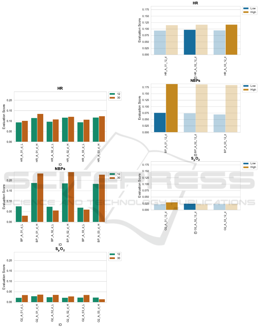
Statistical Models. Figure 1 shows a performance

comparison for all statistical models and all parame-

ters with respect to the train size. We compare train-

ing with 12 lags against training with 30 lags. We em-

ploy a constant sampling frequency of f

= 1 h

−1

be-

cause MIMIC-III does not allow for higher f

. Hence,

Forecasting Thresholds Alarms in Medical Patient Monitors using Time Series Models

12 lags are equivalent to 12 hours of ICU stay and 30

lags are equivalent to 30 hours of ICU stay, respec-

tively. Since there are fewer ICU stays lasting up to

30 hours than ICU stays lasting up to 12 hours, there

are consequently fewer ICU stays to be considered for

the 30 lags train size approach.

Figure 2 compares the statistical models’ perfor-

mance for high alarms against the performance for

low alarms and across the different vital parameters.

There are striking performance differences amongst

parameters and alarm types which will be further dis-

cussed in section 4.

Figure 1: Comparison of train sizes for statistical models

(ARIMA and ARIMAX). For all parameters and model we

compare a train size of 12 lags with a train size of 30 lags

both for high alarms (sufﬁx _H) and low alarms (sufﬁx _L).

Figure 2: Comparison of alarm types (high alarm and low

alarm) for statistical models across all vital parameters.

ML Models. Figure 3 shows a comparison of the

different ML model types, i.e. vanilla RNN, LSTM,

and GRU. The plots show no clear superiority of

one model type. However, the plots suggest that in-

put variables, alarm type, and especially the scal-

ing methods distinctly inﬂuence the models’ perfor-

mance. Hence, we further explore the inﬂuence of the

scaling method in ﬁg. 4. In this ﬁgure, two facts are

to be seen. Firstly, scaling seems to have a distinctly

negative inﬂuence on the model’s performance. This

is most obvious for the SpO

vital parameter but the

effect is also present for HR and NBP

. Secondly,

the type of alarm (high alarm or low alarm) appears

to also have an inﬂuence on the ML models’ perfor-

mances but differently than in the statistical models’

HEALTHINF 2022 - 15th International Conference on Health Informatics

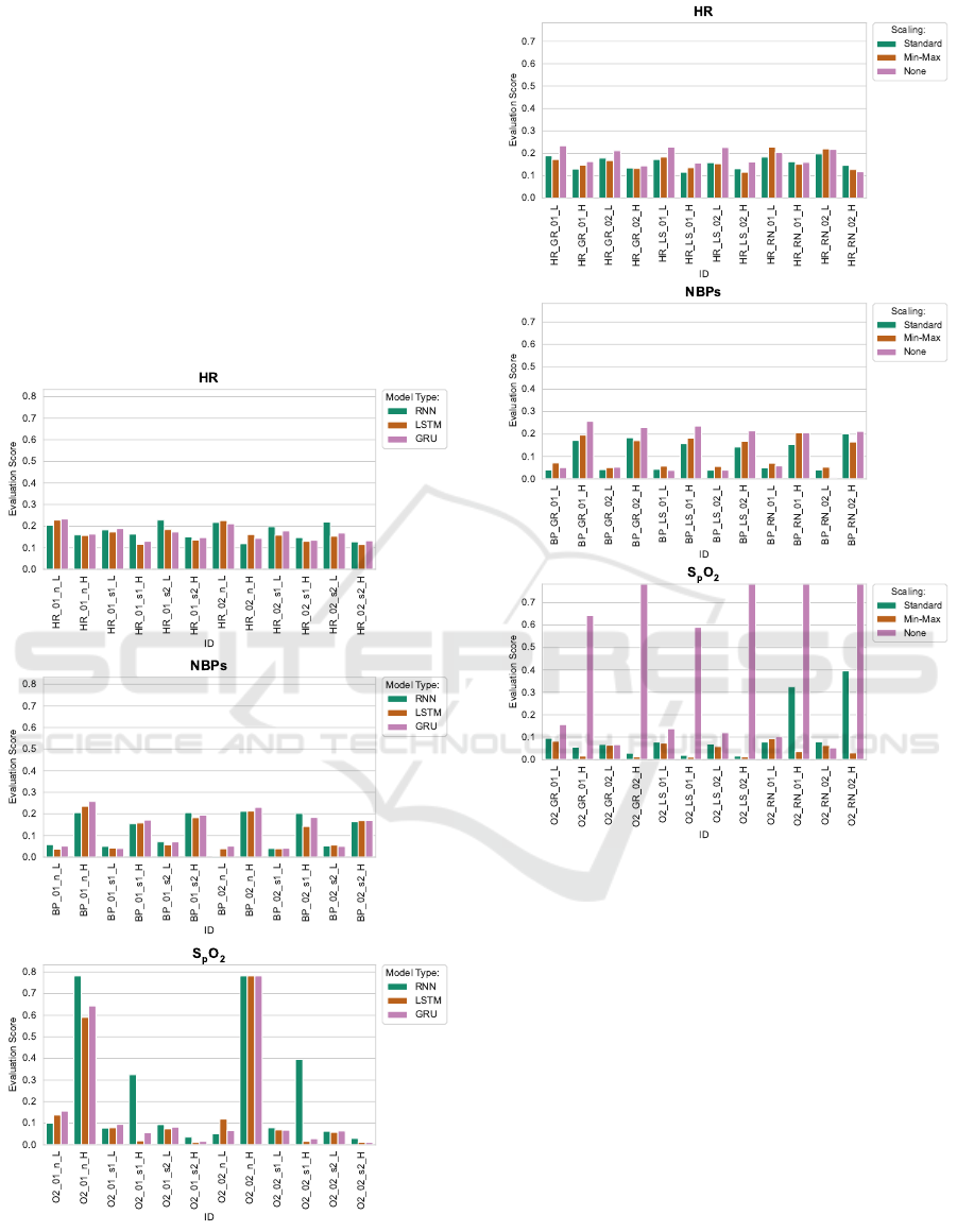
case. For HR, low alarms seem to be forecast slightly

more successfully. For NBP

, high alarms seem to be

forecast distinctly more successfully. For SpO

the

inﬂuence of the scaling method is too high to clearly

see an effect here.

Figure 5 shows an overall comparison of all ML

models and highlights the best performing model for

each combination of vital parameter and alarm type.

For HR and NBP

there is one clear best model con-

ﬁguration for each alarm type. For SpO

, however,

there are multiple best models for the high alarm type.

In general, the GRU model with median resampling

shows the overall best performance according to this

ﬁgure.

Figure 3: Comparison of ML model types vanilla RNN,

LSTM and GRU with different conﬁgurations across vital

parameters and alarm types (sufﬁx _H for high alarms and

sufﬁx _L for low alarms).

Figure 4: Comparison of ML models executed with differ-

ent scaling methods applied (Standard, Min-Max) or with-

out scaling (None) across vital parameters and alarm types

(sufﬁx _H for high alarms and sufﬁx _L for low alarms).

Comparison. Figure 6 compares the best perform-

ing statistical and ML models with each other hav-

ing vital parameter and alarm type as independent

variable. Except for low blood pressure alarms, the

ML models always outperform the statistical models,

most strikingly in the SpO

case.

To give a more in-depth view into the model per-

formances, ﬁg. 7 visualises the confusion matrix for

the best performing models. There, we can see that

the statistical models most prominently produce more

false positives than the ML models. Since our evalua-

tion metric penalises false positives more heavily than

false negatives, this explains the considerably lower

performance of the statistical models in ﬁg. 6.

Forecasting Thresholds Alarms in Medical Patient Monitors using Time Series Models

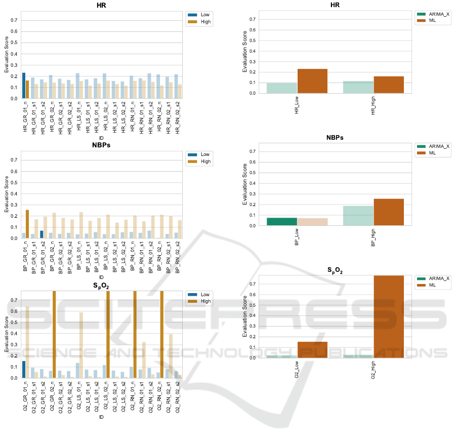
Figure 5: Selection of best ML models. Models with model

type GRU and median resampled chunks as endogenous

input variable always perform best (except for high alarm

forecasting of SpO

4 DISCUSSION

In this paper, we aimed at forecasting threshold

alarms in patient monitors. Therefore, we used the

vital parameter and alarm data as provided by the

MIMIC-III database and employed a wide variety of

forecasting models ranging from statistical models to

machine learning methods. In general, the overall

forecasting performance is not fully satisfactory re-

gardless of the model in use. However, the results

give important insights that can guide further research

into this area which we discuss in the following.

Figure 6: Comparison of best performing statistical models

to best performing ML models.

Train Sizes. In ﬁg. 1 we compare different ARIMA

and ARIMAX models each of which being evaluated

with a train of 12 lags and with a train size of 30 lags

respectively. As a general ﬁnding, longer train sizes

tend to yield better forecasting performance. How-

ever, a longer train size also entails that the patient

needs to stay in the ICU for a longer period of time

before the alarm forecasting model can be used, in

our case 12 hours vs. 30 hours. Another approach

is to raise the time-resolution of the vital parameter

data. With more data points per period of time a larger

train size can be achieved in less time. This mani-

fests future research work and investigations into ICU

databases featuring a higher time resolution, see sec-

tion 4.2.

High and Low Alarms. Figure 2 and ﬁg. 5 show

that model performance vastly differs between high

HEALTHINF 2022 - 15th International Conference on Health Informatics

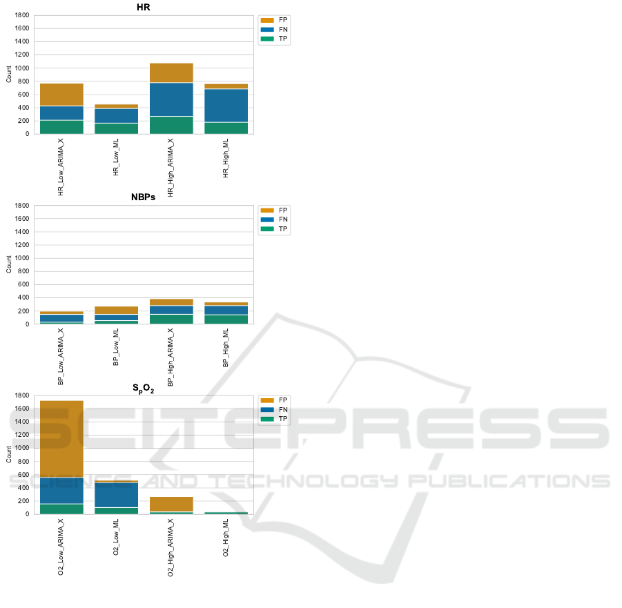
Figure 7: Comparison of confusion matrix values (false

positives, false negatives, and true positives; not showing

true negatives) of best performing statistical models to best

performing ML models.

and low alarms even concerning the same vital pa-

rameter. Especially for HR and NBP

, high alarms are

generally forecast with higher performance regarding

the evaluation score we utilise. Furthermore, peak

forecasting performance for high and low threshold

alarms is not necessarily achieved by the same model.

In the cases of HR and SpO

forecasting, the peak

evaluation score for high alarms is achieved by a dif-

ferent model than the one achieving peak evaluation

performance for the low alarm. Consequently, high

and low alarms of the same vital parameter have to be

considered nonetheless as distinct forecasting tasks.

There is no universal one-ﬁts-all model for threshold

alarm forecasting.

Effects of Scaling. Scaling does not seem to have

a positive effect on the models’ forecasting perfor-

mance, as is to be seen in ﬁg. 4 and ﬁg. 5. In fact,

models using unscaled data consistently exhibit su-

perior or hardly worse performance than their coun-

terparts that do apply scaling methods. An example

where min-max scaling works better than no scaling is

the prediction of alarms of type low in SpO

. We have

no theory on why this is the case. Hence, this man-

ifests a need for further research, ideally in a simpli-

ﬁed forecasting setting (e.g. only forecasting the vital

parameter measurement and no alarms yet) and time

series having a higher and more consistent time reso-

lution, as provided by HiRID and eICU CRD. This is

also described as future work in section 4.2.

Best Performing Models. Figure 6 and ﬁg. 7 show

that amongst the best performing models (both sta-

tistical and ML), the ML models exhibit a superior

performance. This is rooted in the evaluation metric

we utilise that penalises false positives heavier than

false negatives. In ﬁg. 7 it is to be seen that the statis-

tical models tend to produce a higher quantity of false

positives which negatively inﬂuences their scoring in

ﬁg. 6, especially for HR and SpO

4.1 Limitations

In our efforts to forecast threshold alarms in patient

monitors we faced a couple of limitations which we

already mentioned previously and which we want to

summarise here.

Firstly, the relatively low and partially unstable

sampling frequency of the vital parameter measure-

ments poses a problem to our approach. This is two-

fold: On the one hand, the low amount of samples

per period of time forces us to use smaller train sizes

since larger train sizes would correspond to ridicu-

lously long ICU stays. Hence, we have only 12 to

30 lags of training for the statistical models. We as-

sume that this reduces the forecasting performance of

the models since we were able to show that larger

train sizes correspond to better model performance.

On the other hand, the large temporal distance (≈ 1h)

between the samples prevents the forecasting models

from picking up on changes that happen on a more

ﬁne-grained (higher) temporal resolution, potentially

causing false negatives. Higher temporal resolutions

in vital parameter measurements and more detailed

and accurate alarm event data are needed in order to

successfully build accurate alarm forecasting models.

Forecasting Thresholds Alarms in Medical Patient Monitors using Time Series Models

Secondly, our work suggests that each alarm type

requires a dedicatedly tuned model and that there is no

one-ﬁts-all model for forecasting all types of alarms.

Hence, a narrower research focus might be required

for example limiting the forecasting task on one type

of alarms using a more detailed or even specialised

data set.

4.2 Future Work

Forecasting threshold alarms in patient monitors is

basically an extension of forecasting vital parameter

measurements by not only forecasting the value itself

but also comparing the value to the alarm thresholds.

We chose the MIMIC-III database because a unique

feature of this database is that it contains alarm thresh-

olds. However, if we accept that forecasting vital pa-

rameter measurements without accounting for alarms

is a valid preliminary goal, other clinical databases are

eligible as well. For example, HiRID (Hyland et al.,

2020) provides vital parameters measurements with a

vastly higher time resolution and eICU CRD (Pollard

et al., 2018) even provides such data with a steady

sampling frequency of f

5 min

(one value every

ﬁve minutes). This is in sharp contrast to MIMIC-

III which has varying sampling frequencies leaning

towards one value per hour. Using HiRID and eICU

CRD might improve the forecasting accuracy for vi-

tal parameters and also spare us the resampling step

which introduces an additional source of inaccuracies

and errors. Such a simpliﬁed forecasting setting can

then also be used to further investigate the effects of

scaling on the forecasting performance.

5 CONCLUSIONS

The contribution of this paper is a ﬁrst attempt to

forecasting threshold alarms in ICU patient monitors.

Due to the lack of alarm data having a sufﬁciently

high and consistent sampling frequency, the resulting

models are still worthy of improvement and are not

yet ready to be applied in clinical practice. However,

our results show that the general approach of forecast-

ing threshold alarms through vital parameters princi-

pally works and that the model setup used in this work

is promising.

ACKNOWLEDGEMENTS

This work was partially carried out within the

INALO project. INALO is a cooperation project be-

tween AICURA medical GmbH, Charité – Univer-

sitätsmedizin Berlin, idalab GmbH, and Hasso Plat-

tner Institute. INALO is funded by the German Fed-

eral Ministry of Education and Research under grant

16SV8559.

REFERENCES

Clifford, G. D., Silva, I., Moody, B., Li, Q., Kella, D.,

Shahin, A., Kooistra, T., Perry, D., and Mark, R. G.

(2015). The physionet/computing in cardiology chal-

lenge 2015: reducing false arrhythmia alarms in the

ICU. In 2015 Computing in Cardiology Conference

(CinC), pages 273–276. IEEE.

Cvach, M. (2012). Monitor alarm fatigue: an integrative

review. Biomedical instrumentation & technology,

46(4):268–277.

Dai, X., Liu, J., and Li, Y. (2021). A recurrent neural net-

work using historical data to predict time series in-

door PM2.5 concentrations for residential buildings.

Indoor Air.

Drew, B. J., Harris, P., Zègre-Hemsey, J. K., Mammone,

T., Schindler, D., Salas-Boni, R., Bai, Y., Tinoco, A.,

Ding, Q., and Hu, X. (2014). Insights into the problem

of alarm fatigue with physiologic monitor devices: a

comprehensive observational study of consecutive in-

tensive care unit patients. PloS one, 9(10):e110274.

Hyland, S. L., Faltys, M., Hüser, M., Lyu, X., Gumbsch, T.,

Esteban, C., Bock, C., Horn, M., Moor, M., Rieck, B.,

et al. (2020). Early prediction of circulatory failure in

the intensive care unit using machine learning. Nature

medicine, 26(3):364–373.

Johnson, A. E. W., Pollard, T. J., Shen, L., Lehman, L.-

W. H., Feng, M., Ghassemi, M., Moody, B., Szolovits,

P., Celi, L. A., and Mark, R. G. (2016). MIMIC-III, a

freely accessible critical care database. Scientiﬁc data,

3(1):1–9.

Mussumeci, E. and Coelho, F. C. (2020). Large-scale mul-

tivariate forecasting models for dengue-LSTM versus

random forest regression. Spatial and Spatio-temporal

Epidemiology, 35:100372.

Pathan, R. K., Biswas, M., and Khandaker, M. U. (2020).

Time series prediction of COVID-19 by mutation rate

analysis using recurrent neural network-based LSTM

model. Chaos, Solitons & Fractals, 138:110018.

Pollard, T. J., Johnson, A. E., Raffa, J. D., Celi, L. A.,

Mark, R. G., and Badawi, O. (2018). The eICU col-

laborative research database, a freely available multi-

center database for critical care research. Scientiﬁc

data, 5(1):1–13.

HEALTHINF 2022 - 15th International Conference on Health Informatics